Fundamentals of Forecasting

Business Forecasting Methods and Techniques

Descriptive Statistics Analysis
Single & Multiple Moving Averages
Single & Multiple-Parameters Exponential Smoothing
Exponential Smoothing with Seasonality Methods

Decomposition Methods
Simple and Multiple Regression Analysis
Box-Jenkins (ARIMA) Models
Multivariate Data Analysis

Home | About me

Descriptive Statistics Analysis

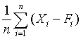
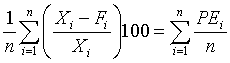
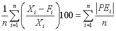
Quantitative forecasts are based on data, or observations. A single observation or actual value can be represented by a variable, X_i ,for example, actual sales $ booked. The objective of forecasting then is to predict the future value of X. Individual forecasts can be denoted by variable F_i ,and the error denoted by e_i which is the difference between actual and forecast value for observation i, for example: e_i = X_i - F_i . In both time-series and casual forecasting, the variable time interval t denotes the present time period, t - 1 last period, t - 2 two periods ago, and so on. Forecasts are for time periods t + 1, t + 2 ... t + m. For the rest of these sections, I will use the following notations.

	Observed	Historical	Present	Forecasted
Values	X₁, X₂ ... X_n	X_t_{- n} ... X_t_{- 2}, X_t_{- 1}	X_t	F_{t + 1} F_{t + 2} ... F_{t + m}
Period i	1, 2 ... 4	t - m ... t - 2, t - 1	t	t + 1, t + 2 ... t + m
Estimated values	F₁, F₂ ... F_n	F - n ... F - 2, F - 1	F_t
Error	e₁, e₂ ... e_n	e_{t - n} ...e_{t - 2}, e_{t - 1}	e_t

Univariate data analysis explores each variable in a data set, separately. It looks at the range of values, as well as the central tendency of the values. It describes the pattern of response to the variable. It describes each variable on its own. Descriptive statistics describe and summarize data. Both Univariate and Bivariate descriptive statistics describe individual variables for the central tendency, variability or dispersion, and shape of the overall distribution.

Bivariate descriptive statistics (e.g., ANOVA, t-tests) often involve more than one quantitative variable being collected and examined. For example, data collected from customers contains kg, feet, locations, dollars spend/week, Return Memo/week. summarizing such data in a way that is analogous to summarizing univariate (single variable) data.

Multivariate descriptive statistics refers to any statistical technique used to analyze data that arises from more than one variable at a time. Multivariate data analysis is about separating the signal from the noise in data with many variables and presenting the results as easily interpretable plots summarizing the essential information. This essentially models reality where each situation, product, or decision involves more than a single variable. A wide range of methods is used for the analysis of multivariate data such as Regression Analysis, Correspondence Analysis, Factor Analysis, Multidimensional Scaling, and Cluster Analysis.

Univariate and Bivariate Data Analysis
	A	B	C	D	E	F	G	H	I
1	Week	Meat sold in Kilogram	Forecast in feet	Deviation From Mean =a_i	Squared Error	Cubed Deviation	Deviation From Mean =e_i	Squared Error e_i²	a_i(e_i)
2	41	3290.8	3119.2	-1019.73	1039849.27	-1060365499.05	-1173.93	1378111.64	1197091.64
3	42	3536.7	3407.1	-773.83	598812.87	-463379362.34	-886.03	785049.161	685636.59
4	43	3902	4073	-408.53	166896.76	-68182333.73	-220.13	48457.2169	89929.71
5	44	4145	4378.9	-165.53	27400.18	-4535551.94	85.77	7356.4929	-14197.51
6	45	4205	4498.9	-105.53	11136.58	-1175243.38	205.77	42341.2929	-21714.91
7	46	4387.9	4199	77.37	5986.12	463145.86	-94.13	8860.4569	-7282.84
8	47	4687.8	4498.9	377.27	142332.65	53697839.96	205.77	42341.2929	77630.85
9	48	4768.8	4498.9	458.27	210011.39	96241921.02	205.77	42341.2929	94298.22
10	49	4936.2	4798.8	625.67	391462.95	244926623.24	505.67	255702.149	316382.55
11	50	5245.1	5458.6	934.57	873421.08	816273143.31	1165.47	1358320.32	1089213.30
		43105.3	42931.3	0	3467309.86	-386035317.05	0	3968881.32	3506987.60
Table 1.1 Statistical Computation for Univariate Data

Go To Top

Table 1.1 above contains both univariate and bivariate data set with values in kilogram, and below are their commonly used descriptive statistics.

Mean, , of volume sold for the past 10 weeks

 =

= 43105.3/10 = 4,310.53 kg

Median (or the middle value)

=5.5, which is value at the 5.5th position =(4205+4387.9)/2 =4296.45 or, =MEDIAN(B2:B11)

Range

Max - Min =MAX(B2:B11)-MIN(B2:B11) =1954.3 kg
The range is very sensitive to extreme scores since it is based on only two values. It should almost never be used as the only measure of spread or dispersion, but can be informative if used as a supplement to other measures of spread such as the standard deviation or semi-interquartile range.

Deviation from the Mean

Xi - 

Note: sum of the deviations always equal to zero, so they should be squared.

Mean Absolute Deviations (MAD)

MAD =

=SUMPRODUCT(ABS(D2:D11))/COUNT(A2:A11) =494.63 kg

Sum of Squared Deviations (SSD)

SSD =

=3,467,309.86 kg

Mean Squared Deviation (MSD)

MSD =

=346,730.98 kg. It is also called the Maximum Likelihood Estimate (MLE).

Variance, var (x) or S², is the sum of squared deviations divided by the degrees of freedom

S² =

=SUM(E2:E11)/(COUNT(A2:A11)-1) =385,256.65 kg

The degrees of freedom (df) can be defined as the number of data points minus the number of parameters estimated (which is 1 in the data kilograms)

S² is closely related to MSD, and because it has a smaller denominator, its value is always larger than MSD. Variance S² is an unbiased estimator of this sample sales variance, whereas MSD is a biased estimator of the sample data variance. (If the mean value of an estimator equals the true value of the quantity it estimates, the estimator is called an unbiased estimator. An estimator is a biased estimator if its expected value is not equal to the value of the population parameter being estimated).

The variance, standard deviation, standard error, as well as the range, all are measuring variability.

Go To Top

Covariance, Cov_xy

cov(x,F) =

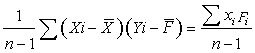
=3506987.60 / 9 =389665.29 kg-feet

Covariance is the measure of how much two variables change together. The covariance becomes more positive for each pair of values which differ from their mean in the same direction. The covariance becomes more negative with each pair of values which differ from their mean in opposite directions (in another word, if one of them tends to be above its expected value when the other variable is below its expected value. (Variance is a special case of the Covariance when the two variables are identical).

Note that the units of covariance, kg-feet, is difficult to interpret. Hence we want to compute the correlation coefficient from Pearson's r which takes care of this scaling problem as described below. If Covariance is divided by the two standard deviations, then the units in the numerator and denominator cancel, leaving with dimensionless number, which will be Pearson's r, the Correlation Coefficient as shown below. Dividing the covariance by the two standard deviations restricts the range r to the interval -1 to +1.

Pearson's product-moment Correlation Coefficient ("ρ" when it is measured in the population and " r " when it is measured in a sample) is a measure of the strength of the linear relationship between two variables. If the relationship between the variables is not linear, then the correlation coefficient does not adequately represent the strength of the relationship between the variables. Simply put it, Correlation Coefficient is the covariance of the deviations of the variables from their means, expressed in terms of their respective standard deviations.

Pearson's r can range from -1 to 1. An r of -1 indicates a perfect negative linear relationship between variables, an r of 0 indicates no linear relationship between variables, and an r of 1 indicates a perfect positive relationship between variables. With real data, you would not expect to get values of r of exactly -1, 0, or -1.

Pearson's correlation is symmetric in the sense that the correlation of X with Y is the same as the correlation of Y with X. A critical property of Pearson's r is that it is unaffected by linear transformations - which means that multiplying a variable by a constant and/or adding a constant does not change the correlation of that variable with other variables. If Y is the transformed value of X, then Y = mX + b.


A perfect linear relationship, Pearson's r = 1	A perfect negative linear relationship, Pearson's r = -1 Note that as X increases, Y decreases.	Scatter plot shows that there is no linear relationship between the variables, Pearson's r = 0.

Pearson's r formula is designed so that the correlation between kilogram and feet (in Table 1.1) is the same whether ’forecast’ is measured in kilogram or in feet.

The value of Pearson's correlation coefficient computed from Table 1.1, is 0.945. So there is a substantial correlation of 0.945 between kilogram and feet, which means there is a strong positive association between the two different set of variables. Hence, the scatter plot chart on the left reveals a strong positive linear relationship between the two variables set.

Covariance and Correlation are closely related statistics to each other in bivariate and especially multivariate data sets. Care must be taken that they are only for measures of linear association and not appropriate for a curvilinear relationship.

Figure 1.0 Scatter Plot Sales and Forecast

Go To Top

Pearson's Correlation Coefficient, r

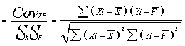
=SUMPRODUCT((D2:D11),(G2:G11))/SQRT(E12*H12)
=3506987.6 / 3709628.2 =0.945

Root Mean Square (RMS)

RMS =

=SQRT(SUM(E2:E11)/COUNT(A2:A11)) =588.84 kg

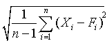
Standard Deviation (SD)
denoted by σ

SD =

=SQRT(SUM(E2:E11)/(COUNT(A2:A11)-1)) =620.69 kg.

Standard Deviation is a measure of the variability or dispersion of a population or a data set. A low standard deviation indicates that the data points tend to be very close to the the mean, while high standard deviation means the data are spread out over a large range of values. It is also commonly used to measure confidence in statistical conclusions

Standard Error of the Mean (SEM)

=STDEV(B2:B11)/SQRT(COUNT(B2:B11)) or, STDEV(B2:B11)/(10^(1/2)) =196.280

SEM is the standard deviation of the error in the sample mean relative to the true mean, since the sample mean is an "unbiased estimator". It is also the standard deviation of the sample mean estimate of a population mean. The standard error of the mean is a "biased estimator" of the population standard error.

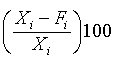
Coefficient of Variation (CV)

CV_X =

CV_F=

=(620.69/4310.53)*100 =14.399

=( 664.07/4293.13) =15.468

=SQRT(SUM(H2:H11)/(COUNT(A2:A11)-1)) =664.07 kg
=SUM(C2:C11)/COUNT(A2:A11) =4293.13 kg

This coefficient provides a unitless measure of the variation of the distribution, by translating it into a percentage of the mean value. This CV value can be used when comparing two parameter samples that have different means and standard deviations. When the mean is close to 0, the CV value becomes of little use.

Skewness

Skew =

= SUMPRODUCT((D2:D11)^3)/(COUNT(D2:D11)-1)*(SQRT(SUM(E2:E11)/(COUNT(E2:E11)-1))^3)

= (-386035317.05) / 9*(620.69)³ = −0.179

Excel, however, uses a slightly different equation for skewness, as shown below. Using Excel's Data Analysis Tool, I obtain the value −0.224. The two results are pretty close.

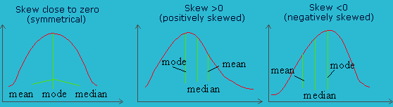
On the right, the positively skewed distribution curve rises rapidly, reaches the maximum and falls slowly; and the tail as well as median on the right-hand side. A negatively skewed distribution curve rises slowly, reaches its maximum and falls rapidly, and the tail as well as the median are on the left-hand side.

Standard Error of Skewness

=SQRT(6/10) =0.775

Measures using Skewness and Kurtosis help to decide normality. Skewness measure indicates the level of non-symmetry. If the distribution of the data are symmetric, then skewness will be close to zero. How can we tell if the skewness is large enough to be a concern? This can be checked using a measure of the standard error of skewness. If the skewness is more than twice this amount, in this case 1.549, then it indicates that the distribution of the data is non-symmetric. However, this does not indicate that the sales data are normally distributed. If Skew is >0, the distribution has a pronounced right tail; whereas if Skew is <0, then the distribution will have a left tail. The sales data distribution shows a negative skewness because the negative deviations dominate the positive deviations, when cubed.

Go To Top

Kurtosis or Kurt(X)

Kurt(X) =

this the Kurtosis formula, but Excel is using a different formula as shown below.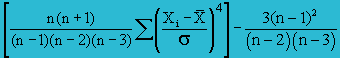

=KURT(B2:B11) = −0.738

Kurtosis is a measure of the peakedness and flatness of the data distribution. Again, for normally distributed data, the kurtosis is zero. Heavier tailed distributions have larger kurtosis measures. The normal distribution has a kurtosis of 0 irrespective of its mean or standard deviation. Positive kurtosis indicates a relatively peaked distribution. Negative kurtosis indicates a relatively flat distribution. As with skewness, if the value of kurtosis is too big or too small, there is concern about the normality of the distribution. In this case, a rough formula for the Standard Error of Kurtosis is =SQRT(24/N) = 0.1.549. Twice this amount is 3.099.

L = Lipto Kurtic (Kurtosis > 0)
M = Meso kurtic (Kurtosis = 0) or a normal distribution
P = Platy kurtic (Kurtosis < 0)

Kurtosis has its origin in the Greek word "Bulginess." Kurtosis is measured relative to the ’peakedness’ or ’flatness’ of the normal curve. It tells us the extent to which a distribution is more peaked or flat-topped than the normal curve.

Go To Top

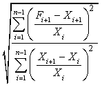
Least-Squares Fitting Technique

Least-Squares Method is used to find the best-fitting curve to a given set of data, $x 1 ... x n$ by minimizing the sum of the squares of the offsets ("the residuals", also called the Sum of Squared Errors or Deviations, SSD) of the points from the curve. Because the sum of the squares of the offsets is used instead of the offset absolute values, outlying points can have a disproportionate effect on the fit, a property which may or may not be desirable depending on the problem at hand. Least-Squares Method can be linear and non-linear, and categorized further as ordinary least squares (OLS), weighted least squares (WLS), and alternating least squares (ALS). Ordinary Linear Least Squares (LLS) fitting technique is the simplest and most commonly applied form of linear regression and provides a solution to the problem of finding the best fitting straight line through a set of points.

Although Excel can plot a trend line instantly for your graphs, but let's use this LLS method as an example to understand the logic and calculation of the coefficients and a straight line that best fits the historical data in Table 1.2 .The equation for the line is: y = mx + b
where the dependent y-value is a function of the independent x-values. The m-values are coefficients corresponding to each x-value, and b is a constant value. Note that y, x, and m can be vectors.

Let X be the number of hours that employees clocked in for work in a typical month, Y be the total units of production output recorded, and there were 11 employees' sample data collected for analysis.

Go To Top

A B C D E F G

1 Monthly Hrs Worked, X_i Monthly Output, Y_i Deviation from Mean
Deviation from Mean

Figure 1.1 Using Linear Least Squares Method to find the best line of ’Fit’ from the example on the left.

2 195 21816 -55.09 -1455.55 80187.32 3035.01

3 279 26893 28.91 3621.45 104692.96 835.74

4 224 20528 -26.09 -2743.55 71581.60 680.74

5 237 20665 -13.09 -2606.55 34122.05 171.37

6 219 21302 -31.09 -1969.55 61234.96 966.64

7 252 24420 1.91 1148.45 2192.50 3.64

8 256 22315 5.91 -956.55 -5652.31 34.92

9 264 19595 13.91 -3676.55 -51137.40 193.46

10 254 25294 3.91 2022.45 7905.96 15.28

11 285 25989 34.91 2717.45 94863.87 1218.64

12 286 27170 35.91 3898.45 139989.96 1289.46

13 Total 2751 255987 0 0 539981.45 8444.91

14 Mean 250.09 23271.55 0 0 49089.22

Table 1.2 Ordinary Least Square Fitting Method to find the best linear Line fit on the bivariate data

Mean of total hours worked
Mean of the monthly output

 =
 =

SUM(B2:B12)/COUNT($B$2:$B$12) =250.09
SUM(C2:C12)/COUNT($B$2:$B$12) =23271.55

The slope m

The intercept, b

Linear Least Squares line LLS

m =

b =

f (X) =

=539981.45 / 8444.91 =63.942 or, use this =INDEX(LINEST(C$2:C$12,B$2:B$12),1)

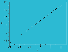
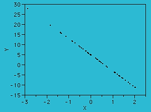
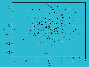
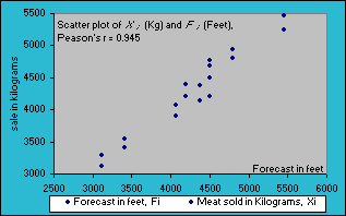
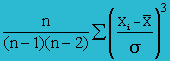
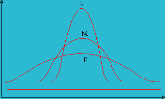
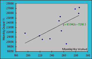
 - m () =23271.55 - 63.942(250.09) =7280.3 or, use this =INDEX(LINEST(C$2:C$12,B$2:B$12),2)

mx + b =63.942x + 7280.3

Table 1.3 Single Time Series lagged On Itself To Determine The Auto-Covariance and Auto-Correlation

	A	B	C	D	E	F	G	H	I	J	K	L	M
1	t		_(k=1)	_(k=2)	_(k=3)		_(k=1)	_(k=2)	_(k=3)
2	1	101				34.05				1159.40
3	2	40	101			-26.95	34.05			726.30	-917.65
4	3	36	40	101		-30.95	-26.95	34.05		957.90	834.10	-1053.85
5	4	116	36	40	101	49.05	-30.95	-26.95	34.05	2405.90	-1518.10	-1321.90	1670.15
6	5	54	116	36	40	-12.95	49.05	-30.95	-26.95	167.70	-635.20	400.80	349.00
7	6	52	54	116	36	-14.95	-12.95	49.05	-30.95	223.50	193.60	-733.30	462.70
8	7	93	52	54	116	26.05	-14.95	-12.95	49.05	678.60	-389.45	-337.35	1277.75
9	8	33	93	52	54	-33.95	26.05	-14.95	-12.95	1152.60	-884.40	507.55	439.65
10	9	77	33	93	52	10.05	-33.95	26.05	-14.95	101.00	-341.20	261.80	-150.25
11	10	64	77	33	93	-2.95	10.05	-33.95	26.05	8.70	-29.65	100.15	-76.85
12	11	43	64	77	33	-23.95	-2.95	10.05	-33.95	573.60	70.65	-240.70	813.10
13	12	59	43	64	77	-7.95	-23.95	-2.95	10.05	63.20	190.40	23.45	-79.90
14	13	27	59	43	64	-39.95	-7.95	-23.95	-2.95	1596.00	317.60	956.80	117.85
15	14	94	27	59	43	-27.05	-39.95	-7.95	-23.95	731.70	-1080.65	-215.05	-647.85
16	15	113	94	27	59	46.05	-27.05	-39.95	-7.95	2120.60	1245.65	-1839.70	-366.10
17	16	109	113	94	27	42.05	46.05	-27.05	-39.95	1768.20	1936.40	1137.45	-1679.90
18	17	69	109	113	94	2.05	42.05	46.05	-27.05	4.20	86.20	94.40	55.45
19	18	39	69	109	113	-27.95	2.05	42.05	46.05	781.20	-57.30	-1175.30	-1287.10
20	19	78	39	69	109	11.05	-27.95	2.05	42.05	122.10	-308.85	22.65	464.65
21	20	42	78	39	69	-24.95	11.05	-27.95	2.05	622.50	-275.70	697.35	-51.15
	sum =	1339								15964.95	-1563.50	-2714.71	1311.24
	mean =	66.95
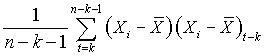
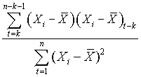
	Auto-Cov (lag 1) = -86.86					Auto-r (lag 1) = - 0.10
	Auto-Cov (lag 2) = - 159.69					Auto-r (lag 2) = - 0.17
	Auto-Cov (lag 3) = 81.95					Auto-r (lag 1) = 0.08

Table 1.3 above is a time series of 20 "equally spaced" data points, denoted by t time period. Each individual data element is referred to as Xt. The mean for the series is x-bar. The data is generated randomly. (hint: you can use this formula to generate a series of random numbers, =INT((85-5+1)* RAND()+5); for this case, I used max=85 and min=5). First, I copy a duplicate of this complete time series to column C but offset by a period of one (time lag k=1). Next I do it similarly in column D and E, lagging the time series by a period each until k=3. Column F is the deviation from the mean. Column G, H, I are basically lagging the deviation of the mean in column F by a lag of one period each. Column J is deviation of the mean squared. Column K is multiplying column F by column G, lagging by one period; column L is column F times column H for 2 periods lagging, and column M is column F times column I for a 3 periods lagging. The calculation of autocovariance and autocorrelation, with one-period lag, is using the following equation:

Auto-Covariance (lag k)

auto-cov_{k
=}

= -1563.50/(20-1-1) = - 86.86

Auto-Correlation (lag k)

auto-r_{k
=}

= -1563.50 / 15964.95 = - 0.10

Using the same equations, you will obtain the result for autocovariance and autocorrelation, for the lag 2, 3 and more periods. The three autocorrelation values (-0.1, -0.17, 0.08) are close to zero, and so we know that there is no clear pattern of linear relationship.

Given a real stochastic process, the autocovariance will be the covariance of the "signal" against a time-shifted version of itself. For example, I want to know "to what extent will the next measurement depend on the data point that I have just examined, or the one that was just before". Auto-covariance would be a measure of this dependence as shown in Table 1.3, with time period offsets. Auto-correlation is simply defined as a normalized form of the auto-covariance. Autocorrelation is the correlation of a data set with itself, offset by k-values. For example, autocorrelation with an offset of 5 would correlate the data set {X1, X2 ... Xn-5} is correlated with {X5, X6 ... Xn}.The autocorrelation function is the set of autocorrelations with offsets 1, 2, 3, 4 ... limit, where limit is <= n/2.

Go To Top


	Table 1.4 Computations of Standard and Relative Statistics on Forecast Errors
	A	B	C	D	E	F	G	H	I	J
1	Period t	Actual Data	Forecast	Forecast Error	Absolute Error	Squared Error	PE	APE	U's numerator	U's denominator
2	1	24	28	-4	4	16	-16.67	16.67	0.085	0.016
3	2	21	28	-7	7	49	-33.33	33.33	0.145	0.510
4	3	36	28	8	8	64	22.22	22.22	0.007	0.007
5	4	33	30	3	3	9	9.09	9.09	0.001	0.008
6	5	36	35	1	1	1	2.78	2.78	0.003	0.012
7	6	40	38	2	2	4	5.00	5.00	0.001	0.010
8	7	44	45	-1	1	1	-2.27	2.27	0.002	0.008
9	8	48	50	-2	2	4	-4.17	4.17	0.002	0.016
10	9	54	52	2	2	4	3.70	3.70	0.005	0.001
11	10	56	52	4	4	16	7.14	7.14
Sum				6	34	168	-6.50	106.38	0.251	0.589

ME	0.60			SDE	4.32
MAE	3.40			SPE	-6.50
SSE	168			MPE	-0.65
MSE	16.8			MAPE	10.63

Theil's U	0.65

Standard Statistical Measures

Go To Top

Mean Error, with n error terms.

ME =

=6/10 =0.6

A low value of the ME may conceal forecasting inaccuracy due to the offsetting effect of large positive and negative forecast errors. But 0.6 in this case is a fair value, given that there are no large typically forecast deviations in the series. However, its inaccuracy will become more apparent from inspection of subsequent forecast evaluation statistics.

Mean Absolute Error

MAE =

=34/10 =3.4

3.4 is a small marginal forecast error, and forecasting has done a good justice. Even though, the MSE and MAE may overcome the 'cancellation of positive and negative errors' limitation of the ME, but in some cases they may fail to provide information on forecasting accuracy relative to the scale of the series being examined, for example when you have multivariate forecast series, F₁ , F₂ , F_3,and more.

Sum of Squared Errors

SSE =

=168

Mean Squared Error

MSE =

=168/10 =16.8

Because MSE squares the errors, and thereby give opportunities to larger errors than does the MAE. This is especially true for the large squared errors (49 and 62) derived from period 2 and 3 respectively, as compared to the sum of squared errors from period 5 through to period 9 (total 14), which are even much smaller. MSE of 16.8 is considered relatively large, and U-statistic can be used to making a comparison.

Standard Deviation Errors

SDE =

=SQRT(168/9) =4.32

Relative Statistical Measures

Go To Top

Percentage Error

PE =

and so SPE, sum of PE = - 6.5

Mean Percentage Error

MPE =

= - 6.5/10 = - 0.65

Mean Absolute Percentage Error

MAPE =

=106.38/10 = 10.64

The objective of using standard statistics and relative statistical measures is often to look for an optimization model so as to minimize the sum or mean of squared errors (MSE, SSE). This may not be a good measure for several reasons. First, the relative measures are giving equal weight to all the time series errors as opposed to MSE, which squares the errors and thereby only emphasizing large errors. Even then, the intention of minimizing MSE to 0 in the fitting phase can always be achieved by using a polynomial of sufficiently high order or an appropriate Fourier transformation. Over-fitting a model to a data series is as good as intentionally including randomness in the generating process, or failing to identify the nonrandom data pattern. Second, because other forecasting methods use different procedures in the fitting phrase -- for example, Smoothing methods are highly dependent on the initial forecasting estimates; Decomposition methods include the trend-cycle in the fitting phase; Regression methods minimize the MSE by giving equal weight to all the collection data points; Box-Jenkins methods minimize the MSE of a non-linear optimization procedure. So, using MSE or SSE as a single criterion alone is rarely adequate. Also, in the forecasting process, using MSE as a measure of statistics accuracy can also create problems. Because MSE is an absolute measure, it does not facilitate comparison across multivariate time series and for different time intervals.

Theil's U-Statistic

Go To Top

U-Statistic

U =

= SQRT(0.251/0.598) =0.65
,which says that naive method can do an equally good forecasting than other formal methods.

U-Statistical measure, although consider as a 'naive' approach to formal forecasting, does in the evaluation process demonstrate a good characteristics of giving more weight to the large errors (which MSE squared to create the disproportionate margins of large errors.) than to the small errors. Theil's U measures how well the forecasting model predicts against a ‘naive’ model. A forecast in a naive model is done by repeating the most recent value of the variable as the next forecasted value. The intervals of the U-statistic can be examined as:

U = 1: The naive estimation approach is as good as the forecasting technique.

U near to 0 : The more accurate the forecasts, the lower the value of the U1 statistic. The U1 statistic is bounded between 0 and 1, with values closer to 0 indicating greater forecasting accuracy. If it is equal to 0 then the forecasting model is a perfect fit.

U < 1: The forecasting technique used demonstrated greater accuracy than the naive method.

U > 1: there is no point in using a forecasting method, since a naive method in this case, produce better results.

In a way, U-statistic provides a good comparison between the formal forecasting methods and the naive forecasting methods.

Demand Forecast Accuracy

Go To Top

Demand Forecast Error is the deviation of the actual realized demand quantity from the forecasted quantity. The Forecast Error can be bigger than Actual or Forecast but NOT both. Error above 100% gets 0% forecast accuracy or a very inaccurate forecast.

Error % = | Actual Demand - Forecast |
Actual Demand

Forecast Accuracy % = 1 - Error %

This site was created in February 2007.
contact Tan, William email: vbautomation@yahoo.com