|
Business Forecasting Methods and Techniques |
Single & Multiple Moving Averages
Single & Multiple-Parameters Exponential Smoothing
Exponential Smoothing with Seasonality Methods
Simple and Multiple Regression Analysis
Box-Jenkins (ARIMA) Models
Multivariate Data Analysis
Exponential Smoothing Methods
Single Exponential
Smoothing (SES)
Adaptive-Response-Rate Single Exponential Smoothing (ARRSES)
Double Exponential Smoothing: Brown's One-Parameter Linear Method
Double Exponential Smoothing: Holt's Two-Parameter Linear Method
The are single, double and more complicated smoothing methods, and all of them share the common property in that recent values are given relatively more weights than the older observations. In another word, weights are exponentially decreasing as observations get older. In the case of moving averages, the weights are by-product of the MA system adopted, but in exponential smoothing, there are one or more smoothing parameters that need to be determined explicitly.
Single Exponential Smoothing
| A simplest case of the Single Exponential Smoothing (SES) can be written as: |
|
(1) | |
|
In equation (1), forecast Ft
+1
is based on weighting the most recent observation Xt
with a weight value of (1-/n) and weighting the most
recent previous forecast Ft
with a weight value of (1-(1/n)). Substituting
|
 |
(2) | |
|
As you see, it is no longer necessary to store
all the historical data as in the case of MA methods. Rather we
only need the most recent observation, the most recent forecast,
and a value for
|
 |
(3) | |
| Repeats this substitution by replacing Ft -1 by its components, we gets equation (4) |
|
(4) | |
| Equations (4)
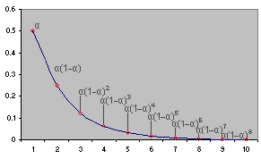
illustrates the exponential behavior. The weights,
|
 |
(5) |
|
Suppose
|
|
The speed at which the older responses are
dampened (smoothed) is a function of the value of
|
|||||||
|
Weight assigned to X: |
|
|
|
|
(1- |
(1- |
(1- |
(1- |
|
|
X t X t -1 X t -2 X t -3 X t -4 X t -5 X t -6 X t -7 X t -8 X t -9 |
.2 .16 .128 .1024 .08192 .065536 .052429 .041943 .033554 (.2)(.8)4 |
.5 .25 .125 .0625 .03125 .015625 .007813 .003906 .001953 (.5)(.5)4 |
.8 .16 .032 .0064 .00128 .000256 .0000512 .00001024 .000002048 (.8)(.2)4 |
0.9 0.7 0.5 0.3 0.1 |
.1 .3 .5 .7 .9 |
.01 .09 .25 .49 .81 |
.001 .027 .125 .343 .729 |
.001 .0081 .0625 .2401 .6561 |
|
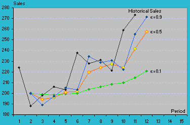
From above illustration, we therefore know that when
![]() has a value
close to 1, the new forecast will include a substantial adjustment for
the error in the previous forecast. When
has a value
close to 1, the new forecast will include a substantial adjustment for
the error in the previous forecast. When
![]() is close to
0, the new forecast will include very little adjustment. SES will always
trail the trend in the actual data, for the most it can do is to adjust
the next forecast for some percentage of the most recent error. Table
1.1 below shows the forecasting for the sales using the
Single Exponential Smoothing.
is close to
0, the new forecast will include very little adjustment. SES will always
trail the trend in the actual data, for the most it can do is to adjust
the next forecast for some percentage of the most recent error. Table
1.1 below shows the forecasting for the sales using the
Single Exponential Smoothing.
|
Table 1.1 Forecasting sales using Single Exponential Smoothing. |
|
Exponentially Smoothed |
Forecast Error |
Absolute Percentage |
Squared Error ( Xi -Fi )2 |
||||||||||||
| Month |
Period t |
Historical Sales Xt | α =0.1 | α =0.5 | α =0.9 | α =0.1 | α =0.5 | α =0.9 | α =0.1 | α =0.5 | α =0.9 | α =0.1 | α =0.5 | α =0.9 | |
| Jan-06 | 1 | 224 | |||||||||||||
| Feb-06 | 2 | 188 | 200 | 200 | 200 | -12 | -12 | -12 | 6.38 | 6.38 | 6.38 | 144.00 | 144.00 | 144.00 | |
| Mar-06 | 3 | 198 | 199 | 194 | 189 | -1 | 4 | 9 | 0.40 | 2.02 | 4.44 | 0.64 | 16.00 | 77.44 | |
| Apr-06 | 4 | 206 | 199 | 196 | 197 | 7 | 10 | 9 | 3.53 | 4.85 | 4.31 | 53.00 | 100.00 | 78.85 | |
| May-06 | 5 | 203 | 199 | 201 | 205 | 4 | 2 | -2 | 1.75 | 0.99 | 1.04 | 12.62 | 4.00 | 4.46 | |
| Jun-06 | 6 | 238 | 200 | 202 | 203 | 38 | 36 | 35 | 16.05 | 15.13 | 14.62 | 1459.00 | 1296.00 | 1210.26 | |
| Jul-06 | 7 | 228 | 204 | 220 | 235 | 24 | 8 | -7 | 10.69 | 3.51 | 2.86 | 594.24 | 64.00 | 42.53 | |
| Aug-06 | 8 | 231 | 206 | 224 | 229 | 25 | 7 | 2 | 10.80 | 3.03 | 1.02 | 621.97 | 49.00 | 5.51 | |
| Sep-06 | 9 | 221 | 209 | 228 | 231 | 12 | -7 | -10 | 5.63 | 2.94 | 4.42 | 154.89 | 42.25 | 95.36 | |
| Oct-06 | 10 | 259 | 210 | 224 | 222 | 49 | 35 | 37 | 19.00 | 13.42 | 14.29 | 2420.73 | 1207.56 | 1370.74 | |
| Nov-06 | 11 | 273 | 215 | 242 | 255 | 59 | 32 | 18 | 21.46 | 11.62 | 6.62 | 3443.44 | 1009.65 | 327.69 | |
| Dec-06 | 12 | 221 | 258 | 272 | |||||||||||
| 95.70 | 63.89 | 60.01 | 8904.53 | 3932.46 | 3356.85 | ||||||||||
| Download SES worksheet |
|
||||||||||||||
| Test Periods | |||||||||||||||
| 2-11 | 2-11 | 2-11 | |||||||||||||
| Statistics Summay: | α =0.1 | α =0.5 | α =0.9 | ||||||||||||
| Mean Error | 20.59 | 11.50 | 7.95 | ||||||||||||
| Mean Absolute Error | 23.15 | 15.20 | 14.03 | ||||||||||||
| Mean Abs. Percentage Error | 9.57 | 6.39 | 6.00 | ||||||||||||
| Standard Deviation of Error | 31.45 | 20.90 | 19.31 | ||||||||||||
| Mean Squared Error | 890.45 | 393.25 | 335.68 | ||||||||||||
One point of concern for SES is the initial estimate values. Since F
Adaptive-Response-Rate Single Exponential Smoothing (ARRSES)
|
The equation for forecasting with
ARRSES method is the same as equation (4) except that
|
|
(6) | |
|
Instead of using
|
where |
(7) (8) (9) (10) |
Table 1.2 Forecasting sales using Adaptive-Response-Rate Single Exponential Smoothing.
|
|
|
|
||||||||||||||||
|
Period t |
Historical Sales |
Forecast Ft |
Error ( ei ) |
Smoothed Error ( Et ) |
Absolute Smoothed Error ( Mt ) |
|
Forecast Ft |
Error ( ei ) |
Smoothed Error ( Et ) |
Absolute Smoothed Error ( Mt ) |
|
Forecast Ft |
Error ( ei ) |
Smoothed Error ( Et ) |
Absolute Smoothed Error ( Mt ) |
|
||
| 1 | 253 | -5.0 | 20.0 | |||||||||||||||
| 2 | 171 | 253.0 | -82.0 | -65.6 | 65.6 | 0.200 | 253.0 | -82.0 | -45.1 | 45.1 | 0.400 | 230.0 | -59.0 | -13.1 | 25.9 | 0.750 | ||
| 3 | 327 | 236.6 | 90.4 | 59.2 | 85.4 | 1.000 | 220.2 | 106.8 | 38.4 | 79.0 | 1.000 | 185.8 | 141.3 | 10.1 | 43.2 | 0.507 | ||
| 4 | 249 | 327.0 | -78.0 | -50.6 | 79.5 | 0.693 | 327.0 | -78.0 | -25.6 | 78.5 | 0.486 | 257.3 | -8.3 | 7.3 | 37.9 | 0.233 | ||
| 5 | 392 | 273.0 | 119.0 | 85.1 | 111.1 | 0.636 | 289.1 | 102.9 | 45.1 | 91.9 | 0.326 | 255.4 | 136.6 | 26.7 | 52.7 | 0.192 | ||
| 6 | 221 | 348.7 | -127.7 | -85.1 | 124.4 | 0.766 | 322.6 | -101.6 | -35.6 | 97.3 | 0.491 | 281.7 | -60.7 | 13.6 | 53.9 | 0.506 | ||
| 7 | 196 | 250.9 | -54.9 | -60.9 | 68.8 | 0.684 | 272.8 | -76.8 | -58.3 | 86.0 | 0.366 | 251.0 | -55.0 | 3.3 | 54.1 | 0.252 | ||
| 8 | 165 | 213.3 | -48.3 | -50.8 | 52.4 | 0.886 | 244.7 | -79.7 | -70.0 | 82.5 | 0.677 | 237.1 | -72.1 | -8.0 | 56.8 | 0.061 | ||
| 9 | 278 | 170.5 | 107.5 | 75.8 | 96.5 | 0.970 | 190.7 | 87.3 | 16.5 | 85.1 | 0.849 | 232.7 | 45.3 | 0.0 | 55.1 | 0.141 | ||
| 10 | 351 | 274.8 | 76.2 | 76.1 | 80.3 | 0.786 | 264.8 | 86.2 | 54.8 | 85.7 | 0.194 | 239.1 | 111.9 | 16.8 | 63.6 | 0.000 | ||
| 11 | 212 | 334.7 | -122.7 | -82.9 | 114.2 | 0.949 | 281.5 | -69.5 | -13.5 | 76.8 | 0.640 | 239.1 | -27.1 | 10.2 | 58.1 | 0.264 | ||
| Test Periods |
With |
|||||||||||||||||
| 2-11 | 2-11 | 2-11 | ||||||||||||||||
| β =0.8 | β =0.55 | β =0.15 | F3 =(0.2*171)+(1-0.2)*253 =236 | |||||||||||||||
| F2 =X1 | F2 =X1 | F2 =230 | e3 =(327-236) =90.4 | |||||||||||||||
| α2 =0.2 | α2 =0.4 | α2 =0.75 | E3 =(0.8*90.4)+((1-0.8)*(-65.6)) =59.2 | |||||||||||||||
| E1= 0 | E1= 0 | E1= - 5 | M3 =(0.8*ABS(90.4)+((1-0.8)*65.6)) =85.4 | |||||||||||||||
| M1= 0 | M1= 0 | M1= 20 | M2 =(0.8*ABS(-82)+((1-0.8)*0)) =65.6 | |||||||||||||||
| Mean Absolute Error: | 90.67 | 87.08 | 44.54 |
|
||||||||||||||
| Mean Squared Error: | 9912.63 | 8585.21 | 7708.39 | F11 =((0.786*351)+((1-0.786)*274.8)) =334.7 | ||||||||||||||
Download
ARRSES woeksheet.
|
|
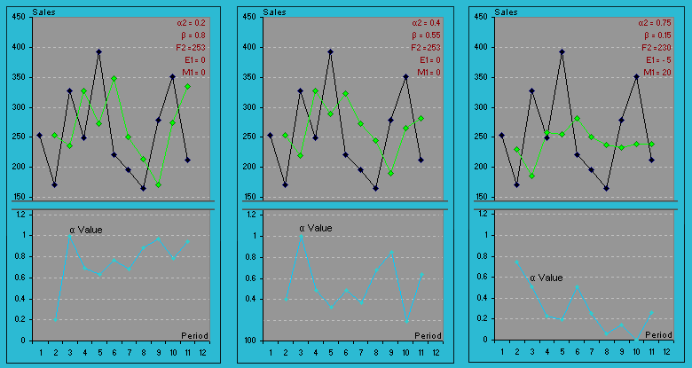
| Figure 1.3 Actual Sales and Forecasts Using Adaptive-response-Rate Single Exponential Smoothing (ARRSES) |
The three graphs plotted in Figure 1.2
are using altogether the different values of
![]() and
and
![]() . Note that
the values of
. Note that
the values of
![]() fluctuate
very differently for all the three scenarios. As you can see it is no
longer true that a smaller value of
fluctuate
very differently for all the three scenarios. As you can see it is no
longer true that a smaller value of
![]() would give
larger effect of smoothing. If you were to use different initializing
values, including the estimate values of F2,
E1
and M1,
entirely different sets of
would give
larger effect of smoothing. If you were to use different initializing
values, including the estimate values of F2,
E1
and M1,
entirely different sets of
![]() values
would have been generated. One way to control the changes in the values
of
values
would have been generated. One way to control the changes in the values
of ![]() is to
change the value of
is to
change the value of
![]() . Note that
when I used a smaller value of
. Note that
when I used a smaller value of
![]() (0.15)
combined with a higher
(0.15)
combined with a higher
![]() (0.75), I
was able to obtain relatively smaller series of
(0.75), I
was able to obtain relatively smaller series of
![]() values; and
simultaneously, a greater smoothing effect had also been achieved for
the forecasts. This is in fact true when looking at the MAE (44.54) and
MSE (7708.4) which have the smallest values among the three.
values; and
simultaneously, a greater smoothing effect had also been achieved for
the forecasts. This is in fact true when looking at the MAE (44.54) and
MSE (7708.4) which have the smallest values among the three.
Summing up, ARRSES is an SES method with
![]() values
systematically changed from period to period to allow for the changes in
the data pattern. Extra care need to be taken when evaluating the
fluctuation in
values
systematically changed from period to period to allow for the changes in
the data pattern. Extra care need to be taken when evaluating the
fluctuation in
![]() . An
alternative is to put an upper bound value on how much
. An
alternative is to put an upper bound value on how much
![]() is allowed
to change (using Excel Conditional Formatting to flag you an alert -
with red fonts, blink, etc) from one period to the
next.
is allowed
to change (using Excel Conditional Formatting to flag you an alert -
with red fonts, blink, etc) from one period to the
next.
Double Exponential Smoothing: Brown's One-Parameter Linear Method
Linear Exponential Smoothing method has great advantages over Linear Moving Averages, mainly because of the limitations of single moving averages that need to save the last n values - more data storage. With Linear Exponential Smoothing, you need to compute only 3 data values and a single value for
The computational rationale of this linear
exponential smoothing is quite similar to linear moving averages - both
the single and double-smoothed values lag the actual data when a trend
exists. The single and double-smoothed values are to be added to the
single smoothed values and then adjust for trend. See the equations
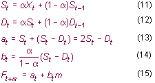
below for the One-Parameter Linear Exponential Smoothing.
| Single exponential smoothed
value is denoted as St
, and Double exponential smoothed value is denoted by
Dt
which will only be computed after values for
St are
determined. at
refers to the adjustment of the St by the
difference of St - Dt
(meaning the adjusted smoothed estimation value for period t). The
trend component
bt
is the estimate of the trend from one time period to another.
Ft
+ m refers
to the derivation of forecast for m
periods ahead of t . The
forecast for m periods ahead
of t is equal to
at
+ bt
(m).
Notice that
at
has a factor of
|
 |
| Table 1.3 Application of Brown's One-Parameter Linear Exponential Smoothing to forecast Sales | ||||||||||||
|
Period t |
Historical Sales |
Single Exponential Smoothing St |
Double Exponential Smoothing Dt |
Value of a |
Value of b |
Value of a+b(m) |
Error Difference ei |
| ei | | ei 2 | APE | ||
| 1 | 125 | 125.00 | 125.00 | |||||||||
| 2 | 149 | 129.80 | 125.96 | 133.64 | 0.960 | |||||||
| 3 | 136 | 131.04 | 126.98 | 135.10 | 1.016 | 134.6 | ||||||
| 4 | 157 | 136.23 | 128.83 | 143.64 | 1.851 | 136.1 | ||||||
| 5 | 173 | 143.59 | 131.78 | 155.39 | 2.952 | 145.5 | ||||||
| 6 | 131 | 141.07 | 133.64 | 148.50 | 1.858 | 158.3 | ||||||
| 7 | 177 | 148.25 | 136.56 | 159.95 | 2.924 | 150.4 | ||||||
| 8 | 188 | 156.20 | 140.49 | 171.92 | 3.929 | 162.9 | ||||||
| 9 | 154 | 155.76 | 143.54 | 167.98 | 3.055 | 175.8 | ||||||
| 10 | 179 | 160.41 | 146.92 | 173.90 | 3.373 | 171.0 | 8 | 7.96 | 63.41 | 4.449 | ||
| T | 11 | 180 | 164.33 | 150.40 | 178.26 | 3.482 | 177.3 | 3 | 2.72 | 7.41 | 1.513 | |
| E | 12 | 150 | 161.46 | 152.61 | 170.31 | 2.213 | 181.7 | -32 | 31.74 | 1007.40 | 21.160 | |
| S | 13 | 182 | 165.57 | 155.20 | 175.94 | 2.592 | 172.5 | 9 | 9.47 | 89.76 | 5.206 | |
| T | 14 | 192 | 170.86 | 158.33 | 183.38 | 3.130 | 178.5 | 13 | 13.47 | 181.49 | 7.017 | |
| 15 | 224 | 181.48 | 162.96 | 200.01 | 4.630 | 186.5 | 37 | 37.49 | 1405.61 | 16.737 | ||
| 16 | 178 | 180.79 | 166.53 | 195.05 | 3.565 | 204.6 | -27 | 26.64 | 709.46 | 14.964 | ||
| P | 17 | 198 | 184.23 | 170.07 | 198.39 | 3.540 | 198.6 | -1 | 0.61 | 0.37 | 0.309 | |
| E | 18 | 206 | 188.58 | 173.77 | 203.40 | 3.703 | 201.9 | 4 | 4.07 | 16.55 | 1.975 | |
| R | 19 | 156 | 182.07 | 175.43 | 188.70 | 1.659 | 207.1 | -51 | 51.10 | 2611.13 | 32.756 | |
| I | 20 | 248 | 195.25 | 179.40 | 211.11 | 3.965 | 190.4 | 58 | 57.64 | 3322.08 | 23.241 | |
| O | 21 | 228 | 201.80 | 183.88 | 219.73 | 4.481 | 215.1 | 13 | 12.92 | 167.02 | 5.668 | |
| D | 22 | 231 | 207.64 | 188.63 | 226.65 | 4.753 | 224.2 | 7 | 6.79 | 46.10 | 2.939 | |
| S | 23 | 175 | 201.11 | 191.13 | 211.10 | 2.497 | 231.4 | -56 | 56.41 | 3181.83 | 32.233 | |
| 24 | 224 | 205.69 | 194.04 | 217.34 | 2.913 | 213.6 | 10 | 10 | 108.21 | 4.644 | ||
| 25 | 220.3 | m=1 | -4 | 329 | 12918 | 175 | ||||||
| 26 | 223.2 | m=2 | ||||||||||
| 27 | 226.1 | m=3 | ||||||||||
| 28 | 229.0 | m=4 | ||||||||||
| 29 | 231.9 | m=5 | ||||||||||
| 30 | 234.8 | m=6 | ||||||||||
| Descriptive Statistics Analysis: | Values: | |||||||||||
| Mean Error | -0.24 | |||||||||||
| Mean Absolute Error | 21.96 | |||||||||||
| MAPE | 11.65 | |||||||||||
| MSE | 861.19 | |||||||||||
| Std Deviation of Error | 30.38 | |||||||||||
| Download worksheet here. |
|
|
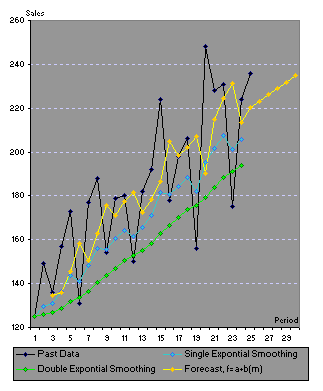
In Table 1.3 the initializing value for
S2
= |
|
Figure 1.4 Applying Forecasts Using Brown's One-Parameter Exponential Smoothing. |
Double Exponential Smoothing: Holt's Two-Parameter Linear Method
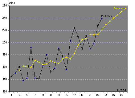
This two-parameter linear
exponential smoothing method is similar in principle to the earlier
one-parameter method. The difference is that it does not apply the
double smoothing formula. It smooths the trend separately by using
different parameters than that used on the original series. There are
two smoothing constants to be used in the equations (![]() and
and ![]() with
values lie between 0 and 1).
with
values lie between 0 and 1).
|
St in equation (16) smooths the
data by helping to eliminate the lag and brings St to the
approximate base of the current data value. Next
bt
updates the trend,
which is expressed as the difference between the last two
smoothed values. This is appropriate because if there is a trend
in the data, new values should be higher or lower than the
previous ones. The constant
|
 |
|
| Table 1.3 shows the
application of this method to a series with trend, using
|
||
| Download worksheet. | ||
|
Table 1.3 Application
of Holt's Two-Parameter Linear Exponential Smoothing ( |
||||||||||
|
Period t |
Historical Sales Xt |
Smoothing Data St |
Smoothing Trend bt |
Forecast F t +m when m=1 |
ei | | ei | | ei 2 | APE | ||
| 1 | 145 | 145.00 | 5.000 | |||||||
| 2 | 150 | 150.00 | 5.000 | |||||||
| 3 | 161 | 156.20 | 5.360 | 155.00 | ||||||
| 4 | 138 | 156.85 | 3.946 | 161.56 | ||||||
| 5 | 142 | 157.04 | 2.819 | 160.79 | ||||||
| 6 | 192 | 166.28 | 4.747 | 159.85 | ||||||
| 7 | 142 | 165.22 | 3.006 | 171.03 | ||||||
| 8 | 141 | 162.78 | 1.372 | 168.23 | ||||||
| 9 | 162 | 163.72 | 1.242 | 164.16 | ||||||
| 10 | 180 | 167.97 | 2.144 | 164.97 | 15 | 15.03 | 225.98 | 8.351 | ||
| T | 11 | 152 | 166.49 | 1.057 | 170.12 | -18 | 18.12 | 328.27 | 11.920 | |
| E | 12 | 158 | 165.64 | 0.484 | 167.55 | -10 | 9.55 | 91.24 | 6.046 | |
| S | 13 | 191 | 171.10 | 1.977 | 166.13 | 25 | 24.87 | 618.73 | 13.023 | |
| T | 14 | 178 | 174.06 | 2.272 | 173.08 | 5 | 4.92 | 24.23 | 2.766 | |
| 15 | 156 | 172.27 | 1.052 | 176.33 | -20 | 20.33 | 413.46 | 13.034 | ||
| 16 | 203 | 179.26 | 2.833 | 173.32 | 30 | 29.68 | 880.96 | 14.621 | ||
| 17 | 224 | 190.47 | 5.348 | 182.09 | 42 | 41.91 | 1756.61 | 18.711 | ||
| P | 18 | 210 | 198.65 | 6.198 | 195.82 | 14 | 14.18 | 201.13 | 6.753 | |
| E | 19 | 189 | 201.68 | 5.247 | 204.85 | -16 | 15.85 | 251.31 | 8.388 | |
| R | 20 | 212 | 207.94 | 5.552 | 206.93 | 5 | 5.07 | 25.71 | 2.392 | |
| I | 21 | 190 | 208.80 | 4.142 | 213.50 | -23 | 23.50 | 552.03 | 12.366 | |
| O | 22 | 198 | 209.95 | 3.246 | 212.94 | -15 | 14.94 | 223.14 | 7.544 | |
| D | 23 | 228 | 216.16 | 4.134 | 213.20 | 15 | 14.80 | 219.16 | 6.493 | |
| 24 | 239 | 224.03 | 5.256 | 220.29 | 19 | 19 | 350.04 | 7.828 | ||
| 25 | 229.29 | m=1 | 67 | 271 | 6162 | 140 | ||||
| 26 | 234.55 | m=2 | ||||||||
| 27 | 239.80 | m=3 | ||||||||
| 28 | 245.06 | m=4 | ||||||||
| 29 | 250.31 | m=5 | ||||||||
| 30 | 255.57 | m=6 | ||||||||
| S23 =0.2(X23)+((1 - 0.2)(S22+b22) | Descriptive Statistics Analysis: | Values: | ||||||||
| S23 =0.2*(228)+(0.8*(209.95+3.25)) =216.16 | Mean Error | 4.46 | ||||||||
| b23 =0.3(S23 - S22)+((1 - 0.3)b22 | Mean Absolute Error | 18.10 | ||||||||
| b23 =0.3(216.16 - 209.95)+(0.7*(3.25)) =4.138 | Mean Abs. Percentage Error (MAPE) | 9.35 | ||||||||
| F24 =S23+b23(1) =216.16+4.138 =220.29 | Mean Squared Error (MSE) | 410.80 | ||||||||
| F27 =S24+b24(3) =224.03+(5.256*3) =239.80 | Std Deviation of Error | 20.98 | ||||||||
 |
||||||||||
|
|
||||||||||
This site
was created in February 2007.
contact Tan, William email:
vbautomation@yahoo.com
