|
Business Forecasting Methods and Techniques |
Single & Multiple Moving Averages
Single & Multiple-Parameters Exponential Smoothing
Exponential Smoothing with Seasonality Methods
Simple and Multiple Regression Analysis
Box-Jenkins (ARIMA) Models
Multivariate Data Analysis
Multiple Moving Averages
In the previous section, I mentioned using the Mean as an unbiased estimator that minimizes mean-squared error (MSE) of actual-minus-forecast values. The Mean can be a useful statistic or forecast for the next period(s) only if a time series is generated by a constant process subject to random errors. However, if the data series involve a trend or seasonal effect, or a combination of both, then the Mean is no longer able to capture such patterns. So in this and the next section I will explain using Multiple Moving Averages and a variety of Smoothing methods that can improve upon the Mean to be used as a forecasting measure for the future periods. For the start, let's get familiarized with the forecasting scenario as shown below.
| Xt |
: Xt means the observed data at the current period t |
| Ft |
: Ft means the fitted values (using a forecasting model) at current period t |
| Data set covering the last n time periods | : X1 X2 X3 ...... Xn - 1 Xn |
| Past Data for n time periods | : Xt - n + 1 ...... Xt - 2 Xt - 1 Xt |
| Future Forecasts required for m periods | : Ft + 1 Ft + 2 ..... Ft + m |
| Fitted Values using a forecasting model | : Ft - n + 1 ...... Ft - 2 Ft - 1 Ft |
| Fitting Errors | : (Xt - n + 1- - Ft - n + 1) ...... (Xt - 1 - Ft - 1) (Xt - Ft) |
|
Forecasting Errors (when
Xt
+ 1 .... Xt + m
become available) |
: (Xt + 1 - Ft + 1) , (Xt + 2 - Ft + 2) ..... (Xt + m - Ft + m) |
Once a forecasting model is selected, we fit the model to the known data
(by your choice of parameters and initializing procedures) and obtain
the fitted values. We than calculate the fitted errors, and as
new new observations become available we examine the forecasting errors.
Moving averages are mostly recursive in nature - moving through the past
data period by period, as opposed to using all the past data in one
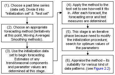
fitting such as in least squares fitting. Figure 2.1 shows a 6 stages
procedure that is used to appraise any forecasting methods.
|
The Single Moving Average of the latest n observations has a few drawbacks in that it gives equal weightage to the observation data; and also it can not handle trend and seasonality very well, although it can forecast better than the Mean. Double Moving Average (or moving averages of moving averages) ends up with unequally weighted averages, and can be used within a method called linear moving averages. The method using Double Moving Averages applies an unequal weights to the past data, and because the weights typically decay in an exponential manner from the most recent to the most distant data point, the method is often called Exponential Smoothing methods. All Smoothing methods require that certain parameters be defined (their values lie between 0 and 1). I will explain on Exponential Smoothing methods in the next page. |
|
|
||||||
| Pulse |
With Random Error |
No Trend Effect |
No Seasonal Effect | Additive Seasonal | Multiplicative Seasonal | |
 |
 |
 |
 |
|||
| Ramp |
 |
Additive Trend |
 |
 |
 |
|
| Step |
 |
Multiplicative Trend |
 |
 |
 |
|
|
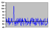
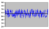
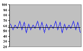
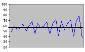
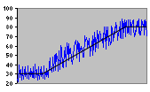
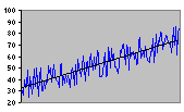
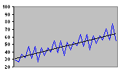
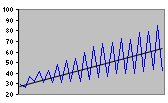
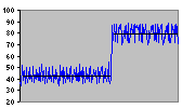
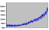
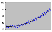
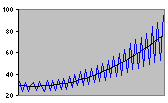
Figure 2.2 Some Common Test Patterns For Testing Forecasting Procedures |
||||||
Single Moving Averages
The term moving average means using a method of computation when each new observation data point becomes available, a new average is then computed by dropping the oldest observation point and including the new one. This moving average will then be the forecast for the next period. To illustrate this, let's say there are N data points and a decision to use t observations for each average (I call it moving average of order t, or simply MA (t). Statistically, it can be shown as below:
| Initialization Set | Test Set | |
| X1 X2 ...... Xt | Xt + 1 Xn | |
|
Time |
Moving Average | Forecast |
| t |
|
Ft + 1
=
 |
| t + 1 |
|
Ft +
2 =
 |
Table 2.1 below illustrates using
a 3-month, 4-month and a 12-month Moving Average method
to forecast a time series of product sales, based on past 24 months data
points.
| Month |
Period t |
Historical Sales Qty Xt |
3-Month Moving Average MA(3) |
4-Month Moving Average MA(4) |
12-Month Moving Average MA(12) |
||
| Jan-06 | 1 | 200 | - | - | - |
 |
|
| Feb-06 | 2 | 135 | - | - | - | ||
| Mar-06 | 3 | 195 | - | - | - | ||
| Apr-06 | 4 | 197 | 176.7 | - | - | ||
| May-06 | 5 | 310 | 175.7 | 181.8 | - | ||
| Jun-06 | 6 | 175 | 234.0 | 209.3 | - | ||
| Jul-06 | 7 | 155 | 227.3 | 219.3 | - | ||
| Aug-06 | 8 | 130 | 213.3 | 209.3 | - | ||
| Sep-06 | 9 | 220 | 153.3 | 192.5 | - | ||
| Oct-06 | 10 | 277 | 168.3 | 170.0 | - | ||
| Nov-06 | 11 | 235 | 209.2 | 195.5 | - | ||
| Dec-06 | 12 | 210 | 244.2 | 215.5 | - | ||
| Jan-07 | 13 | 161 | 240.9 | 235.5 | 203.3 | ||
| Feb-07 | 14 | 146 | 202.2 | 220.8 | 200.0 | ||
| Mar-07 | 15 | 208 | 172.5 | 188.0 | 200.9 | ||
| Apr-07 | 16 | 256 | 171.9 | 181.3 | 202.0 | ||
| May-07 | 17 | 180 | 203.5 | 192.8 | 206.9 | ||
| Jun-07 | 18 | 234 | 214.9 | 197.5 | 196.1 | ||
| Jul-07 | 19 | 190 | 223.5 | 219.5 | 201.0 | ||
| Aug-07 | 20 | 132 | 201.5 | 215.0 | 203.9 | ||
| Sep-07 | 21 | 124 | 185.5 | 184.0 | 204.1 | ||
| Oct-07 | 22 | 295 | 148.9 | 170.0 | 196.1 | ||
| Nov-07 | 23 | 212 | 183.9 | 185.3 | 197.6 | ||
| Dec-07 | 24 | 185 | 210.5 | 190.8 | 195.7 | ||
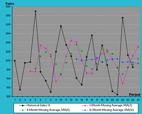
| Jan-08 | 25 | - | 230.9 | 204.0 | 193.6 | Figure 2.3 Actual and Moving Average Values for 12-Months Data | |
| Test Periods | |||||||
| Month 4 -24 | Month 5 - 24 | Month 12 - 24 | |||||
|
Mean |
198.18 3.34 60.35 28.89 71.95 4930.57 1.01 -0.95 |
198.66 3.09 55.44 30.99 68.12 4408.93 0.97 -0.81 |
200.63 -7.04 42.43 24.15 53.63 2636.82 0.84 -1.01 |
||||
Here are the workout of the moving averages as the forecast:
April-06's forecast at MA(3) =
(200+135+195) / 3 = 176.7
May-06's forecast at MA(3) = (135+195+197) / 3
May-06's forecast at MA(4) = (200+135+195+197) / 4
= 181.8
Jan-08's forecast at MA(12) = the average for
Jan-07 through to Dec-07
Comparing Ft + 1 (176.7) and Ft + 2 (175.7) in MA(3), the value of Ft + 2 requires dropping X1 (200) and adding Xt + 1 (197), so another way of know Ft + 2 is:
Ft + 2 = Ft + 1 + (Xt + 1 - X1) / t = 176.7+((197-200)/3) = 175.7
Some points to observe here as to what number of t periods you would choose for the moving average. MA(1) - a moving average of order 1 - taking the last known data as the next period's forecast is truly impractical. Using MA(3) or MA(4) would effectively smooth out seasonal effects (especially for additive seasonal data pattern) as shown in Figure 2.3 above, but if it is used as a forecast for the next period, it self will not be able to accommodate trend or seasonality pattern. However, you can use MA(4) as a Centered Moving Average rather than as a forecast, to help to examine the deviations, spreads and other components within the time series.
MA(12) or larger, as you can see in Figure 2.3, would smooth seasonal effects out of the time series, and would be useful in decomposing the series into trend, seasonal and other components (explained in the next page). Again, if used on its own, is not very useful as a forecasting tool for data that exhibits trend and seasonality. The larger the order of the moving averages, the greater the smoothing effect, and the lesser attention it pays to the fluctuations in the series.
In the above chart, you can see that a small value of t in MA(t) allows the moving averages to follow the pattern, and these MA forecasts can trail the pattern by lagging behind one or a few periods.
Double Moving Averages
The Double Moving Average method (or 2nd moving averages of the 1st -order moving averages) gives you unequally weighted averages, and intended to handle data series with trend better than the single moving averages. Double-Moving Average can be denoted as MA (M x N) which means an M-period MA of an N-period MA. In order to mitigate against the systemic error that occurs when moving averages are applied to data series with trend, we therefore use a method called linear moving averages. Table 2.2 below shows you a few ways of forecasting the series with trend pattern, using a MA(MxN) Linear Moving Average.
| (1) | (2) | (3) | (4) | (5) | (6) | (7) | (8) | (9) | |||
| Month |
Period t |
Historical Sales Xt |
4-Month Moving Average of (1) MA(4) |
Error Difference (1st adjustment) (1) - (2) |
4-Month Moving Average of (2) MA(4X4) |
Error Difference (2nd adjustment) (2) - (4) |
Double-MA Adjusted Forecast (2) + (5) |
Value of a |
Value of b |
Value of a+b(m) when m = 1 |
|
| Jan-06 | 1 | 140 | |||||||||
| Feb-06 | 2 | 159 | |||||||||
| Mar-06 | 3 | 136 | |||||||||
| Apr-06 | 4 | 157 | 148.0 | 9.0 | |||||||
| May-06 | 5 | 173 | 156.3 | 16.8 | |||||||
| Jun-06 | 6 | 131 | 149.3 | -18.3 | |||||||
| Jul-06 | 7 | 177 | 159.5 | 17.5 | 153.3 | 6.3 | 165.8 | 4.2 | |||
| Aug-06 | 8 | 188 | 167.3 | 20.8 | 158.1 | 9.2 | 165.8 | 176.4 | 6.13 | 169.9 | |
| Sep-06 | 9 | 154 | 162.5 | -8.5 | 159.6 | 2.9 | 176.4 | 165.4 | 1.92 | 182.6 | |
| T | Oct-06 | 10 | 179 | 174.5 | 4.5 | 165.9 | 8.6 | 165.4 | 183.1 | 5.71 | 167.3 |
| H | Nov-06 | 11 | 180 | 175.3 | 4.8 | 169.9 | 5.4 | 183.1 | 180.6 | 3.58 | 188.8 |
| E | Dec-06 | 12 | 160 | 168.3 | -8.3 | 170.1 | -1.9 | 180.6 | 166.4 | -1.25 | 184.2 |
| Jan-07 | 13 | 182 | 175.3 | 6.8 | 173.3 | 1.9 | 166.4 | 177.2 | 1.29 | 165.1 | |
| T | Feb-07 | 14 | 192 | 178.5 | 13.5 | 174.3 | 4.2 | 177.2 | 182.7 | 2.79 | 178.5 |
| E | Mar-07 | 15 | 224 | 189.5 | 34.5 | 177.9 | 11.6 | 182.7 | 201.1 | 7.75 | 185.5 |
| S | Apr-07 | 16 | 188 | 196.5 | -8.5 | 184.9 | 11.6 | 201.1 | 208.1 | 7.71 | 208.9 |
| T | May-07 | 17 | 198 | 200.5 | -2.5 | 191.3 | 9.3 | 208.1 | 209.8 | 6.17 | 215.8 |
| Jun-07 | 18 | 206 | 204.0 | 2.0 | 197.6 | 6.4 | 209.8 | 210.4 | 4.25 | 215.9 | |
| P | Jul-07 | 19 | 203 | 198.8 | 4.3 | 199.9 | -1.2 | 210.4 | 197.6 | -0.79 | 214.6 |
| E | Aug-07 | 20 | 238 | 211.3 | 26.8 | 203.6 | 7.6 | 197.6 | 218.9 | 5.08 | 196.8 |
| R | Sep-07 | 21 | 228 | 218.8 | 9.3 | 208.2 | 10.6 | 218.9 | 229.3 | 7.04 | 224.0 |
| I | Oct-07 | 22 | 231 | 225.0 | 6.0 | 213.4 | 11.6 | 229.3 | 236.6 | 7.71 | 236.4 |
| O | Nov-07 | 23 | 221 | 229.5 | -8.5 | 221.1 | 8.4 | 236.6 | 237.9 | 5.58 | 244.3 |
| D | Dec-07 | 24 | 259 | 234.8 | 24.3 | 227.0 | 7.8 | 237.9 | 242.5 | 5.17 | 243.5 |
| S | Jan-08 | 25 | 273 | 246.0 | 27.0 | 233.8 | 12.2 | 242.5 | 258.2 | 8.13 | 247.7 |
| Feb-08 | 26 | 274.4 | |||||||||
| Mar-08 | 27 | 282.6 | |||||||||
| From Test Periods 10 to 25 | |||||||||||
| MA(4) | MA(4X4) |
Double-MA Adjusted Forecast |
a+b(m) when m =1 |
||||||||
| Mean Absolute Error (MAE) | 11.95 | 16.88 | 16.36 | 18.04 | |||||||
| Mean Abs. Percentage Error (MAPE) | 5.39 | 7.62 | 7.66 | 8.62 | |||||||
| Mean Squared Error (MSE) | 241 | 466.77 | 404.54 | 431.64 | |||||||
| Standard Deviation of Error | 16.03 | 22.31 | 20.77 | 21.46 | |||||||
| Table 2.2 Forecasting a Series With Trend Using Linear Moving Average | |||||||||||
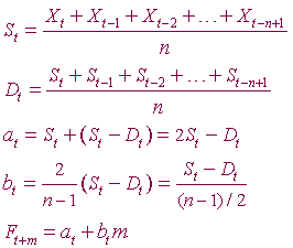
The general Linear Moving Average has the following equations, from which the series in Table 2.2 are computed:
 |
For
Equations on the left, Single-Moving Average, MA(N), is denoted
as St .The
Double-Moving Averages are denoted as Dt
and will only compute when all the single-MA
averages are computed.
at
refers to the adjustment of the single-MA, St
by the difference St - Dt ,
meaning the adjusted smoothed value for period t. The
trend component bt
is the estimate of the trend from one time period to another.
The last equation
Ft
+ m refers
to how to obtain forecasts for m
periods ahead of t . The forecast for
m periods ahead is equal to
at
+ bt
(m).
Note that 2/(n-1) in bt arises because n period of moving average should be centered at a time period (n+1)/2. For instance, the first moving average at n time period for MA(4) is using n - (n+1)/2 which is the difference of (n-1)/2 or (4-1)/2 =1.5 periods. For n =4, as in periods _1___2_x_ 3___4_ the cross mark is where 1.5 periods (i.e. correction for lag) should be centered, and MA(4) is computed at period 4. |
See below for a few workout examples from Table 2.2:
4-Month MA, MA(4) value at period 4
= (140+159+136+157) / 4
4-Month Double-MA, MA(4X4) value at period 7 =
(148.0+156.3149.3+159.5) / 4
Double-MA Adjusted Forecast at period 10, F10 =
[MA(4) at period 9] + [MA(4) - MA(4X4) at period 9]
=
(162.5+(162.5-159.6)) = 165.4
Adjusted smoothed value for period 10,
a10
= 2(174.5)-165.9 =183.1
Trend Estimate for period 24, or b24
= 2(234.8 - 227)/(4-1) = 5.17
Forecast a+b(m) with m=1 for
period 25, Ft
+ 25
= a24
+ b24
(1) = 242.5 + 5.17 = 247.7
Forecast a+b(m) with m=2 for
period 26, Ft
+ 26
= a25
+ b25
(2) = 258.2 + 8.13(2) =
274.4
Forecast a+b(m) with m=3 for
period 27, Ft
+ 27
= a26
+ b26
(3) = 258.2 + 8.13(3) =
282.6
Download worksheet for Table 2.2.
|
|
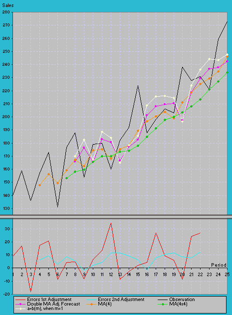
The 2nd Error Adjustment, MA(4) - MA(4X4), is most effective when the series has a linear trend, and the random error component is not strong. But when significant random error is present, it will not always possible to improve on the Single-MA forecast by applying a Linear-MA method as shown in Figure 2.4 on the left. The double-moving averages MA(4X4) provides a better smoothing than the single-MA method, MA(4). This can be further seen in the first and second adjustment lines of of the errors difference. The 2nd errors adjustment (the light blue line) was able to smooth out most of the the random errors characterized in the series. The forecast values (the pink line curve, represented by column 6 in Table 2.2) does look like a good compromise between the methods of MA(4X4) and forecast with f =a+b(m), after it was adjusted by the errors difference between MA(4) and MA(4X4). When compared, its summary statistics, MAE (16.3), MAPE (7.66), and MSE (404.5) show that the means are lower, and it does smooth out some extreme random errors, and still able to trail the trend in the series pretty well. It can be considered a good forecasted series. By no means you should be restricted by using a proportionate 3 X 3 or a 4 X 4 MA system. There is no reason not to try a 3 X 4 or even a 3 X 5 X 5 X 7 MA system (a three-period MA of a five-period MA of a five-period MA of a seven-period MA of data series) if you believe that the few historical months or years of data are still significantly reliable). One point to note is that all moving averages methods imply a set of weights for the past n data points. See below an illustration on the unequal weightings implied for X data series in a MA(3X3) double-MA: S1 =
(X1+X2+X3) / 3 , S2
=(X2+X3+X4) / 3, S3
=(X3+X4+X5) / 3 |
|
Figure 2.4 Application of Linear Moving Averages as a Forecast |
This site
was created in February 2007.
contact Tan, William email:
vbautomation@yahoo.com
