AutoFilters
and Advanced Filters
The
syntax of the AutoFilter property is:
expression.AutoFilter(Field, Criteria1, Operator, Criteria2,
VisibleDropDown)
| expression | Required. It returns one of the objects in the Applies To list. |
| Field | Optional Variant. The integer offset of the field on which you want to base the filter (from the left of the list; the leftmost field is field 1) |
| Criteria1 | Optional Variant. The criteria (a string; for example, "021"). You can use "=" or "<>" for your find. If this argument is omitted, the criteria is All. |
| Operator |
Optional.
XlAutoFilterOperator can be one of these constants: xlAnd (default) xlBottom10Items xlBottom10Percent xlOr xlTop10Items xlTop10Percent Use xlAnd and xlOr with Criteria1 and Criteria2 to construct compound criteria. |
| Criteria2 | Optional Variant. The second criteria (a string). Used with Criteria1 and Operator to construct compound criteria. |
| VisibleDropDown | Optional Variant. True to display the AutoFilter drop-down arrow for the filtered field. False to hide the AutoFilter drop-down arrow for the filtered field. True by default. |
Note: If you omit all the arguments, this method simply toggles the display of the AutoFilter drop-down arrows in the specified range.
T
his code below will filter a list starting in cell A1 on Sheet1 to display only the entries in which field 1 is equal to the string "AMSEA". The drop-down arrow for field 1 will be hidden.
Worksheets("Sheet1").Range("A1").AutoFilter
field:=1, Criteria1:="AMSIA", _
VisibleDropDown:=False ‘
hide the AutoFilter drop-down arrow. To unhide, set it to True
The following example sets the variable
‘c1’ to the value of the Criteria1 property of the filter for the
first column in the filtered range on sheet1.
With Worksheets("sheet1")
If .AutoFilterMode Then
With .AutoFilter.Filters(1)
If .On Then c1 = .Criteria1
End With
End If
End With
For this example, you must first make sure that all
filters are off. It uses “IF...Then” statement to display the current
status of the AutoFilterMode property on your active sheet.
If the AutoFilterMode property is True, the next code would disactivate
the AutoFilter in your active sheet.
If ActiveSheet.AutoFilterMode = True Then
Selection.AutoFilter
' or
use ActiveSheet.AutoFilterMode = False
If ActiveSheet.FilterMode = True Then
ActiveSheet.ShowAllData
End If
End If
This
example filters column A for unique values and copy to one after the
last column on the same worksheet.
Dim LastRowcell As Range, LastColCell As Range
Set LastRowcell = Cells.Find("*", , , , xlByRows, xlPrevious)
Set LastColCell = Cells.Find("*", , , , xlByColumns, xlPrevious)
If Not LastRowcell Is Nothing Then
Range(Cells(1, 1), Cells(LastRowcell.Row, 1)).AdvancedFilter _
Action:=xlFilterCopy, CopyToRange:=Cells(1, LastColCell.Column + 1),
_
Unique:=True
End If
Input this Event
procedure in Sheet1. In this example, the Part Numbers are located in
Column A in both Sheet1 and Sheet2, but in column B in Sheet3. With reference to the Part Number in
Sheet1, and you want to check the shipping detail of the specific part number in Sheet2
and its unit selling price in Sheet3. Simply double-click any part number in
Sheet1, it will bring you to where you want to see.
DOWNLOAD worksheet example here.
Private Sub Worksheet_BeforeDoubleClick(ByVal Target As Range, Cancel As
Boolean)
Dim cellSEL
If ActiveCell.Column = 1 Then
cellSEL = ActiveCell.Value
Sheets("Sheet2").Select
If ActiveSheet.AutoFilterMode = False Then
Selection.AutoFilter
End If
If Not IsNumeric(Right(cellSEL, 1)) Then
Selection.AutoFilter Field:=1,
Criteria1:="=*" & Mid(cellSEL, 1, Len(cellSEL) - 1) & "*", Operator:=xlAnd
Else
Selection.AutoFilter Field:=1,
Criteria1:="=*" & cellSEL & "*", Operator:=xlAnd
End If
Sheets("Sheet3").Select
If ActiveSheet.AutoFilterMode = False Then
Selection.AutoFilter
End If
If Not IsNumeric(Right(cellSEL, 1)) Then
Selection.AutoFilter Field:=2,
Criteria1:="=*" & Mid(cellSEL, 1, Len(cellSEL) - 1) & "*", Operator:=xlAnd
Else
Selection.AutoFilter Field:=2,
Criteria1:="=*" & cellSEL & "*", Operator:=xlAnd
End If
End If
End Sub
AdvancedFilter Method
It filters or copies data from a list based on a criteria range. If the
initial selection is a single cell, that cell's current region is used.
The syntax is:
expression.AdvancedFilter(Action, CriteriaRange, CopyToRange, Unique)
| expression | Required. An expression that returns one of the objects in the Applies To list. |
| Action |
Required
XlFilterAction. can be one of these constants:
xlFilterCopy xlFilterInPlace |
| CriteriaRange | Optional Variant. The criteria range. If this argument is omitted, there are no criteria. |
| CopyToRange | Optional Variant. The destination range for the copied rows if Action is xlFilterCopy. Otherwise, this argument is ignored. |
| Unique | Optional Variant. True to filter unique records only. False to filter all records that meet the criteria. The default value is False. |
T

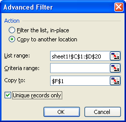
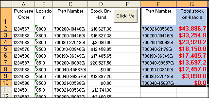
One of the useful features of AdvancedFilter is able to extract a unique list of one field from a range of dataset. The example shows how to obtain a unique list of Part Numbers from a dataset, knowing that Part Number is in column C. Of course, you should use Find method to locate C1 s ActiveCell so as not to hardcode it, but for this example, let’s bear with hardcoding C1. The unique list is copied to the last column but offset by 2, sort by ascending order. Add a header and calculate using R1C1 style formula, which is the equivalent of spreadsheet array function as “=sumproduct(($C$2:$D$30=F2)*($D$2:$D$30))”. Then it copies the array formula to all blank cells in column G (until the row in column F where unique list is blank). Diagram below is the exact output of what you should be seeing after this procedure is run. You can DOWNLOAD the worksheet example.
Sub GetUniqueList_AdvFilter()
Dim inRng As Range, outRng As Range
Dim finalrow As Long, finalcolumn2ToRight As Long
Dim finalrowUnq As Long, finalrowUnq2 As Long
' Identify size of dataset
finalrow = Cells(65536, 1).End(xlUp).Row
finalcolumn2ToRight = Cells(1, 255).End(xlToLeft).Offset(, 2).Column
' Copy C1
heading to last cell in row 1, offset by 2 columns to the Right
‘ In a non-static user environment, you would want this value to be
passed from input box or userform such as:
‘ i = InputBox("Enter the header address you want to be copied to")
‘ Then use this line Range(i).Copy Destination:=Cells(1,
finalcolumn2ToRight)
Range("C1").Copy Destination:=Cells(1, finalcolumn2ToRight)
' Define
output range and input range
Set outRng = Cells(1, finalcolumn2ToRight)
Set inRng = Range("C1").Resize(finalrow, finalcolumn2ToRight - 2)
' Use
AdvancedFilter to obtain the unique Part Numbers list.
It could also be written as inRng.AdvancedFilter xlFilterCopy, outRng,
True
inRng.AdvancedFilter Action:=xlFilterCopy, CopyToRange:=outRng,
unique:=True
'
Identify number of unique part numbers
finalrowUnq = Cells(65536, finalcolumn2ToRight).End(xlUp).Row
' Sort
the the unique dataset
Cells(1, finalcolumn2ToRight).Resize(finalrowUnq, 1).Sort key1:=Cells(1,
_
finalcolumn2ToRight), order1:=xlAscending, header:=xlYes
' Give a
header title
Cells(1, finalcolumn2ToRight + 1).Value = "Total stock on-hand $"
' Add an
array formula to get the Totals.
' Excel spreadsheet equivalent is =SUMPRODUCT(($C$2:$D$30=F2)*($D$2:$D$30))
Cells(2, finalcolumn2ToRight + 1).FormulaArray = _
"=sumproduct((R2C3:R" & finalrow & "C4=RC[-1])*(R2C4:R" & finalrow &
"C4))"
' Copy
array formula to all blank cells in column G (until the row in column F
where unique list is blank)
Cells(2, finalcolumn2ToRight + 1).Copy Cells(3, finalcolumn2ToRight + 1)
_
.Resize(finalrowUnq - 2, 1)
' Format
a range
Range("IV1").End(xlToLeft).Offset(1, 0).Select
Range(ActiveCell, ActiveCell.End(xlDown)).Rows.Select
With Selection
.Font.Size = 10
.Font.ColorIndex = 3
.Font.Bold = True
.NumberFormat = "$#,##0.0"
End With
' Sort by
Total stock on-hand $ in descending order
finalrowUnq2 = Cells(65536, ActiveCell.Column).End(xlUp).Row
Rows("1:1").Find(What:="$", SearchDirection:=xlNext).Activate
ActiveCell.Offset(, -1).Resize(finalrowUnq2, 2).Select
Selection.Sort Key1:=ActiveSheet.Rows("1:1").Find(What:="$", _
SearchDirection:=xlNext), Order1:=xlDescending, Orientation:=xlTopToBottom
End Sub
From the
above code, in fact you would notice that the key in extracting a unique
list is to copy the header in C1 to a blank cell F1, and set this blank
cell address as output range. Thus you can simplify a part of your code
like below.
Range("F1").Value = Range("C1").Value
Range("C1").Resize(finalrow, finalcolumn2ToRight - 2).AdvancedFilter
xlFilterCopy, CopyToRange:=Range("F1"), unique:=True

A note on the NumberFormat Property
This property applies to the DataLabel, DataLabels, PivotField, Style, and TickLabels objects. For the PivotField object, you can set the NumberFormat property only for a Data area field. Take note that the Format function uses different format code strings than do the NumberFormat and NumberFormatLocal properties.
These examples below set the number format for cell A2:A1000, column 2, and column C to F on Sheet1.
Worksheets("Sheet1").Range("A2:A1000").NumberFormat = "General"
Worksheets("Sheet1").Columns(2).NumberFormat = "hh:mm:ss"
‘ Shows
number format in red font and in parenthesis
Worksheets("Sheet1").Columns("C").NumberFormat =
"$#,##0.00_);[Red]($#,##0.00)"
‘ Use a
single comma and include “K” character suffix to indicate numbers are in
thousands, eg. $12,345.6K
Worksheets("Sheet1").Columns("C").NumberFormat = "$#,##0.0,K"
‘ Prefix
the “M” character with a backlash. “M” indicates numbers in millions, eg.
123.45678 thus becomes $123.456M
Worksheets("Sheet1").Columns("C").NumberFormat = "$#,##0.000 \M"
‘ Shows
the number format in billions, eg. 1234567 thus becomes $1.23B
Worksheets("Sheet1").Columns("C").NumberFormat = "$#,##0.00,,""B"""

