Automating Pivot Tables

You usually create your pivot table from the Excel User Interface by choosing from Data menu item: Data>PivotTable and PivotChart Report Wizard, but you can also use VBA to create pivot table such as when you want to automate your routine summary report.

Figure 1.1 Click on the Layout button will bring you to the Pivot Table Layout dialog as shown in the next diagram



 

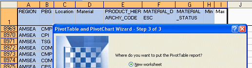
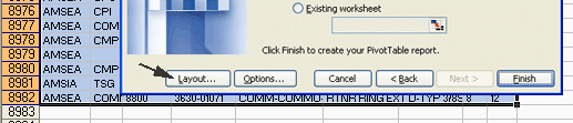
Figure 1.2  You can drag Field names from the right-hand side and drop them in the Row, Column, and Data areas of the PivotTable and PivotChart Report Wizard Layout dialog.

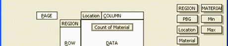
Figure 1.3  When you are done, click OK, then click Finish, and almost instantly, Excel creates a summary of the data that you want to see.




 

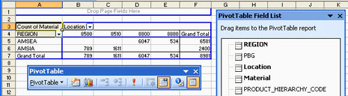
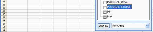
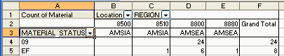
Figure 1.4 below shows another field ‘MATERIAL_STATUS’ was added to the Row area of the pivot table. You can add and remove other fields as you like to the Row, Column, and Data areas. You can move REGION to the Top, or to the Right, or to the Column, all depends on your need.

CreatePivotTable method 

The following example demonstrates an auto-creation of pivot table using VBA. In Excel 2000 and newer versions, you would first build a PivotCache object to input the data range. After the pivot table is defined, you use CreatePivotTable method to input pivot table output destination and pivot table name, and with this you create a blank pivot table based on your defined PivotCache.  In the .AddFields method, you can specify one or more fields that you want to include in the Row, Column, or Data area of the pivot table. To add a field (‘Material’ as in this example) to the Page Data area of the pivot table, you would change Orientation property of the field to xlDataField.

' Define input area and set up a pivot cache
Dim wsh As Worksheet, rng As Range, lastRow As Long, pt as PivotTable
lastRow = ActiveSheet.Cells(65536, 1).End(xlUp).Row
Set wsh = Worksheets("sheet1")
Set rng = wsh.Cells(1, 1).Resize(lastRow, 9)

' Delete any prior pivot tables
On Error Resume Next

For Each pt In wsh.PivotTables

    pt.TableRange2.Clear   ' TableRange2 refers to cell range of the entire pivot table

Next pt

ActiveWorkbook.PivotCaches.Add(SourceType:=xlDatabase, SourceData:= _
  rng.Address).CreatePivotTable TableDestination:=Sheets.Add.Cells(3, 1), _
  TableName:="PivotTable"

' Set up the Row and Column fields
ActiveSheet.PivotTables("PivotTable").AddFields RowFields:="Material_Status" _
  , ColumnFields:=Array("Location", "Region")

' Set up the Data field
ActiveSheet.PivotTables("PivotTable").PivotFields("Material").Orientation = _
  xlDataField

‘ Setting the Function property to xlSum allow you to use summation instead of using xlCount
ActiveSheet.PivotTables("PivotTable").PivotFields("Count of Material").Function = xlSum

‘ At this point, if you set the ManualUpdate to False, Excel calculates. You can immediately thereafter set it back to True
pt.ManualUpdate = False
pt.ManualUpdate = True

Here is the code:

Dim ws As Worksheet, wsh As Worksheet, pt As PivotTable, pc As PivotCache
Dim rng As Range, lastRow As Long, wba As Workbook, wsp As Worksheet
lastRow = ActiveSheet.Cells(65536, 1).End(xlUp).Row
Set ws = Worksheets("sheet1")
Set rng = ws.Cells(1, 1).Resize(lastRow, 9)

On Error Resume Next
For Each pt In ws.PivotTables
  pt.TableRange2.Clear  'TableRange2 refers to cell range of the entire pivot table
Next

Set pc = ActiveWorkbook.PivotCaches.Add(SourceType:=xlDatabase,SourceData:=rng.Address)
Set pt = pc.CreatePivotTable(TableDestination:=Sheets.Add.Range("A3"),
    TableName:="myPivotTable")

‘ To change the orientation of the pivot fields
With pt
   .PivotFields("Material").Orientation = xlDataField
   .PivotFields("Region").Orientation = xlRowField
   .PivotFields("Material_Status").Orientation = xlRowField
   .PivotFields("Location").Orientation = xlColumnField
End With

pt.PivotFields("Region").Subtotals(1) = False ' suppressing the subtotals for multiple column fields
pt.ColumnGrand = False   ‘ suppressing the Grand Total for rows
pt.RowGrand = True       ' set to False will suppress the Grand Total for Columns

Set wba = Workbooks.Add(xlWBATWorksheet)   ‘ create a new workbook to hole the pivot table report
Set wsp = wba.Worksheets(1)
wsp.Name = "summary report"       ‘ give the first worksheet in the new workbook a title
pt.TableRange2.Offset(1, 0).Copy  ‘ use Offset(1,0)  to avoid copy the title row of the pivot table

‘ copy the pivot table data to row 1 of the new report sheet
wsp.[A1].PasteSpecial Paste:=xlPasteFormulasAndNumberFormats
pt.TableRange2.Clear  ‘ erase the original pivot table
Set pc = Nothing      ‘ dissociate variable ‘pc’  from the object.

Note: if you want to have zeros instead of blanks in the Data area of the pivot table, use the following line:

pt.NullString = "0"

Filling in the blank Outline view in column A

If you had been using reports obtained pivot tables, you would notice this blank Outline view which are quite meaningless, usually in column A [see sample].  Here is a simple code that would let you fill in all those blank with the cell above it. See this sample output after you have executed the code.

Option Explicit
' Using pivot table to create a summary report, move around cells and formatting
Sub CreatePivotTable_SummaryReport()
Dim wsd As Worksheet
Dim pRange As Range
Dim ptCache As PivotCache
Dim pt As PivotTable
Dim finalrow As Long, finalcolumn As Long
Set wsd = Worksheets("sheet1")

A note on Sort Method
 
It sorts a PivotTable report, a range, or the active region if the specified range contains only one cell.

Key2 Optional Variant. The second sort field, as either text (a PivotTable field or range name) or a Range object. If you omit this argument, there’s no second sort field. Cannot be used when sorting Pivot Table reports.