Charting with VBA
Charts CollectionIt is the collection of all the chart sheets in a workbook. Each chart sheet is represented by a Chart object. This doesn’t include charts embedded on worksheets or dialog sheets. The collection has an Add method which adds a new chart sheet (Chart1 by default) to the workbook.
This example below adds a new chart sheet (named “MyChart1”) to the active workbook and places the new chart sheet immediately after the worksheet named Sheet1. See the diagram below, and note that the plot area of the chart sheet is grey color by default. The code specifies the data source for the new chart, using SetSourceData method, where Source is the range reference and PlotBy is a constant which be either values: xlColumns or xlRows. This is the same thing as when you right-click the chart, select “Source Data” from the shortcut menu [see sample]. The third line specifies the ‘to-be-created’ chart to be located as a new chart sheet, and give new chart sheet a name “MyChart1”. This third line is put to use when you want to change the embedded chart, on whichever sheet, to a chart sheet or vice versa. The Location method is the equivalent of when you right-click a chart, selecting “Location” from the shortcut menu [see sample].
 |
 |
 |
 |
 |
 |
 |
 |
 |
 |
 |
 |
Charts.Add After:=Worksheets("Sheet1")
ActiveChart.SetSourceData Source:=Sheets("sheet1").Range("A1:B5"),
PlotBy:=xlColumns
ActiveChart.Location Where:=xlLocationAsNewSheet, Name:="MyChart1"
Charts("MyChart1").SizeWithWindow = True
’ or you can use ActiveChart.Location xlLocationAsNewSheet, "MyChart1"
To activate the chart sheet “MyChart1”, you would use:
Sheets("MyChart1").Activate
Column chart is
the default chart type in Excel, and although you can leave out PlotBy:=
xlColumns, it is not a good idea because the user may have set his
default chart type to a line chart or pie chart, and it doesn’t
serve your purpose. SizeWithWindow Property sets MyChart1 to be sized to
its window.
The Location method has this syntax:
expression.Location(Where, Name)
| expression | Required |
| Where |
Required
XlChartLocation. Where to move the chart. XlChartLocation can be one of these XlChartLocation constants: xlLocationAsNewSheet xlLocationAsObject xlLocationAutomatic |
| Name | Optional Variant; required if Where is xlLocationAsObject. The name of the sheet where the chart will be embedded if Where is xlLocationAsObject or the name of the new sheet if Where is xlLocationAsNewSheet. |
Using Object
Variablee
Using object
variables can make your code more efficient and with variables you can
refer to a chart without actually activating it. That means you define
an object variable as Charts object and each time you will only have to
refer to that variable instead of typing long sentences. For example,
instead of using:
Dim ob As Object
charts.Add
ActiveChart.ChartType = xlColumnClustered
ActiveChart.SetSourceData Source:=Sheets("Sheet1").Range("A1:B5")
ActiveChart.Location Where:=xlLocationAsObject, Name:="Sheet1"
Set ob = Worksheets("Sheet1").ChartObjects(1)
With ob.Chart
.HasTitle = True
‘adds a title to the first embedded chart on Sheet1
.ChartTitle.Text = "My 1st chart using VBA"
End With
you can define an object variable as a chart by using this:
Dim c As Chart
Set c = charts.Add
c.SetSourceData Source:=Sheets("Sheet1").Range("A1:B5")
With ActiveChart
.ChartType = xlColumnClustered
.HasTitle = True
.ChartTitle.Text = "My 1st chart using VBA"
.Location Where:=xlLocationAsObject, Name:="Sheet1"
End With
This examples below
is more flexible in terms of my control over the output because
ChartObjects.Add requires me to state the position and size of the
chart.
With ActiveSheet.ChartObjects.Add(Left:=55, Top:=3, Width:=190,
Height:=115)
.Chart.SetSourceData Source:=Sheets("Sheet1").Range("A1:B5")
.Chart.ChartType = xlColumnClustered
End With
’
following are the formatting on chart title, X and Y series axis, legend
and data plot area
Dim ob As Object
Set ob = Sheets("Sheet1").ChartObjects(1)
With ob.Chart
.HasTitle = True
.ChartTitle.Text = "I moved my chart"
.ChartTitle.Font.Name = "Arial"
.ChartTitle.Font.Size = 9
.ChartTitle.Top = 1
.ChartTitle.Left = 30
End With
With ob.Chart.Axes(xlValue, xlPrimary)
'
xlValue as row & primary axis
.HasTitle = True
.AxisTitle.Text = "quantity"
.AxisTitle.Font.Size = 8
.AxisTitle.Left = 1
.AxisTitle.Top = 35
.TickLabels.AutoScaleFont = True
.TickLabels.Font.Size = 8
.HasMajorGridlines = True
.HasMinorGridlines = False
.MinimumScaleIsAuto = True
.MaximumScaleIsAuto = True
.MinorUnitIsAuto = True
.MajorUnitIsAuto = True
End With
With ob.Chart.Axes(xlCategory)
'
xlCategory as column axis
.HasTitle = True
.AxisTitle.Text = "week"
.AxisTitle.Font.Size = 8
.TickLabels.Font.Size = 8
End With
With ob.Chart.Legend
.Font.Size = 8
.Left = 145
.Top = 36
End With
With ob.Chart.PlotArea
.Left = 17
.Top = 10
.Height = 90
.Width = 118
End With
Axes Method
Returns an
object that represents either a single axis or a collection of the axes
on the chart. The syntax is:
expression.Axes(Type,
AxisGroup)
Type
is optional and specifies the axis to return. Can be one of the
following XlAxisType constants:
xlValue, xlCategory, or xlSeriesAxis
(xlSeriesAxis is valid only for 3-D charts).
AxisGroup
is optional XlAxisGroup, and specifies the axis group. If
this argument is omitted, the primary group is used.
3-D charts have only one axis group. XlAxisGroup can be one of these
XlAxisGroup constants:
xlPrimary as default
xlSecondary
Chart Property
Returns a Chart object that represents the chart contained in the
object.
ChartObjects Method
Returns an object that represents either a single embedded chart or a
collection of all the embedded charts.
ChartArea Property
Returns a ChartArea object that represents the complete chart area for
the chart.
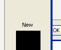
In this example, you notice that the sizing handle becomes to black, indicating that you have selected the ChartArea inside the ChartObjects in active sheet. See the diagram illustration below.
ActiveSheet.ChartObjects(1).Activate
ActiveChart.ChartArea.Select
ChartArea Object
Represents the chart area of a chart. It contains the chart title and
the legend; it doesn’t include the plot area (the area within the chart
area where the data is plotted). The following example sets the pattern
for the chart area in embedded chart one on the worksheet named
"Sheet1."
Dim Ob As Object
Set Ob = Worksheets("sheet1").ChartObjects(1)
With Ob.Chart.ChartArea
.Interior.Pattern = xlLightDown
.Fill.Visible = True
.Fill.ForeColor.SchemeColor = 16
.Fill.BackColor.SchemeColor = 2
End With
SeriesCollection
Collection
Object
Use the SeriesCollection method to return the SeriesCollection
collection.
Use SeriesCollection.Extend method to add the data in cells C1:C5
on Sheet1 to an existing series in the series collection in embedded
chart one on Sheet1.
Worksheets("Sheet1").ChartObjects(1).Chart.SeriesCollection.Extend _
Worksheets("Sheet1").Range("C1:C5")
SeriesCollection.Add method adds the data from cells C1:C5 as a new
series on the embedded chart one on Sheet1.
Worksheets("Sheet1").ChartObjects(1).Chart.SeriesCollection.Add Source:=
_
Worksheets("Sheet1").Range("C1:C5")
This
example clears the formatting of embedded chart one on Sheet1.
ChartWizard
Method
It modifies the
properties of the given chart. You can use this method to quickly format
a chart without setting all the individual properties. The syntax is:
expression.
ChartWizard(Source, Gallery, Format, PlotBy, CategoryLabels, SeriesLabels,HasLegend, Title, CategoryTitle, ValueTitle, ExtraTitle)
|
expression |
Required. An expression that returns one of the objects in the Applies To list. |
|
Source |
Optional Variant. The range that contains the source data for the new chart. If this argument is omitted, Microsoft Excel edits the active chart sheet or the selected chart on the active worksheet. |
|
Gallery |
Optional
XlChartType |
|
Format |
Optional Variant. The option number for the built-in autoformats. Can be a number from 1 through 10, depending on the gallery type. If this argument is omitted, Microsoft Excel chooses a default value based on the gallery type and data source. |
|
PlotBy |
Optional Variant. Specifies whether the data for each series is in rows or columns. Can be one of the following XlRowCol constants: xlRows or xlColumns. |
|
CategoryLabels |
Optional Variant. An integer specifying the number of rows or columns within the source range that contain category labels. Legal values are from 0 (zero) through one less than the maximum number of the corresponding categories or series. |
|
HasLegend |
Optional Variant. True to include a legend. |
|
Title |
Optional Variant. The chart title text. |
|
CategoryTitle |
Optional Variant. The category axis title text. |
|
ValueTitle |
Optional Variant. . The value axis title text |
|
ExtraTitle |
Optional Variant. The series axis title for 3-D charts or the second value axis title for 2-D charts. |
This example
using ChartWizard method to reformat the first embedded chart as a line
chart, adds a legend, and adds category and value axis titles.
ActiveSheet.ChartObjects(1).Width = 170
ActiveSheet.ChartObjects(1).Chart.ChartWizard Gallery:=xlLine, _
HasLegend:=True, CategoryTitle:="Week", ValueTitle:="Qty Delivered"
This example sets
the chart area interior color of Chart1 to Grey and sets the border
color to Red. You have to reference the Chart object inside the
ChartObjects object.
With ActiveSheet.ChartObjects(1).Chart.ChartArea
.Interior.ColorIndex = 15
.Border.ColorIndex = 3
End With
PlotArea
Object and LineStyle Property
The plot
area is surrounded by the chart area. The chart area contains the axes,
the chart title, the axis titles, and the legend. LineStyle property
sets the line style for the border. The following code places a dashed
red border around the chart area, places a continuous thick white border
around the plot area, sets X and Y axis title font size, and formatting
the legend.
ActiveSheet.ChartObjects(1).Activate
With ActiveChart
.ChartArea.Border.LineStyle = xlDash
.ChartArea.Interior.ColorIndex = 15
.Axes(xlValue).AxisTitle.Font.Size = 8
.Axes(xlCategory).AxisTitle.Font.Size = 8
With .PlotArea.Border
.LineStyle = xlContinuous
.Weight = xlThick
.ColorIndex = 2
End With
With .Legend
.Border.LineStyle = xlAutomatic
.Border.Weight = xlHairline
.Shadow = True
.Interior.ColorIndex = 35
.Interior.PatternColorIndex = 1
.Interior.Pattern = xlSolid
.Font.Size = 8
.Font.FontStyle = "Italic"
.Font.Bold = True
End With
End With
XlLineStyle
can be one of these XlLineStyle constants:
xlContinuous
xlDash
xlDashDot
xlDashDotDot
xlDot
xlDouble
xlSlantDashDot
xlLineStyleNone
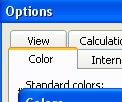
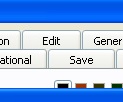
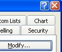
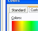
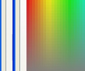
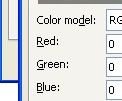
RGB Function
The
Format dialog box displays a default palette of 56 colors to choose
from, but you can define your own color pallet by choosing from menu
Tool/Options/Color, and click Modify, then Custom. Your modified pallet
is saved with the active workbook. All colors can be derived from the
RGB function (Red,Green,Blue) as shown in the diagram below. For pure
red, the RGB equivalent would be RGB(255,0,0). Thus, instead of using:
.Border.ColorIndex = 3
.Border.ColorIndex = RGB(255,0,0)
 |
 |
 |
 |
 |
 |
 |
 |
 |
 |
 |
 |
 |
 |
 |
 |
Data Series
Each
series in a chart is a member of the SeriesCollection collection.
In my example, the chart has two data series, which is “ABC” and “XYZ”.
The code below would change the “ABC” data series to a Line Type, set a
thin line weight, and place diamond markers pf size 8
Dim s As Series
Set s = Worksheets("sheet1").ChartObjects(1).Chart.SeriesCollection("ABC")
With s
.ChartType = xlLine
.Border.Weight = xlThin
.MarkerStyle = xlDiamond
.MarkerBackgroundColorIndex = xlAutomatic
.MarkerForegroundColorIndex = xlAutomatic
.MarkerSize = 8
End With
Putting it all
together
This
example is the final automation procedure that put together the
different pieces which I have shown you in the previous examples. It
adds a chart object in Sheet1 with chart type Line-Column on 2 axes and
position to the position I want; adds a title, primary Y-axis title;
defines line as thin with diamond markerstyle; adds a secondary Y-axis
title and format the secondary axes using TickLabels.NumberFormat;
assign major gridlines to the chart plot area and also adjust the plot
area position; apply data labels in the chart to display value and
adjust their font size, font color; position legend to the right; and
finally save the chart in GIF format to a specified directory.
charts.Add
ActiveChart.ApplyCustomType ChartType:=xlBuiltIn, TypeName:="Line -
Column on 2 Axes"
ActiveChart.Location Where:=xlLocationAsObject, Name:="Sheet1"
With ActiveChart
.Parent.Left = 185
.Parent.Width = 510
.Parent.Top = 8
.Parent.Height = 225
.HasTitle = True
.ChartTitle.Text = "Putting it together"
.ChartTitle.Top = 1
.ChartTitle.Left = 160
.Axes(xlCategory, xlPrimary).HasTitle = True
.Axes(xlCategory, xlPrimary).AxisTitle.Text = "Inaccessible inventory"
.Axes(xlValue, xlPrimary).HasTitle = True
.Axes(xlValue, xlPrimary).AxisTitle.Text = "Total $Cost"
End With
Dim s As Series
Set s = Worksheets("sheet1").ChartObjects(1).Chart.SeriesCollection("%")
With s
.AxisGroup = xlSecondary
.ChartType = xlLine
.Border.Weight = xlThin
.MarkerStyle = xlDiamond
.MarkerBackgroundColorIndex = xlAutomatic
.MarkerForegroundColorIndex = xlAutomatic
.MarkerSize = 8
End With
Dim sA As Axis
Set sA = Sheets("sheet1").ChartObjects(1).Chart.Axes(xlValue, xlSecondary)
With sA
.HasTitle = True
.AxisTitle.Caption = "%"
.TickLabels.NumberFormat = "00.0"
End With
ActiveChart.PlotArea.Select
With ActiveChart.Axes(xlValue)
.HasMajorGridlines = True
.HasMinorGridlines = False
End With
With ActiveChart.Axes(xlCategory)
.HasMajorGridlines = False
.HasMinorGridlines = False
End With
With ActiveChart.PlotArea
.Top = 15
.Height = 200
End With
ActiveChart.ApplyDataLabels AutoText:=True, LegendKey:=False, _
HasLeaderLines:=False, ShowSeriesName:=False, ShowCategoryName:=False, _
ShowValue:=True, ShowPercentage:=False, ShowBubbleSize:=False
With ActiveChart
.SeriesCollection(1).DataLabels.Font.Size = 8
.SeriesCollection(2).DataLabels.Font.Size = 8
.SeriesCollection(2).DataLabels.Font.ColorIndex = 3
End With
ActiveChart.HasLegend = True
ActiveChart.Legend.Select
Selection.Position = xlRight
ActiveChart.HasDataTable = False
Dim c As Chart
Set c = Sheets("Sheet1").ChartObjects(1).Chart
c.Export Filename:="C\temp\MyFirstChart.gif", filtername:="gif"
 |
 |
 |
 |
 |
 |
 |
 |
 |
 |
 |
 |
ChartType
Property
Excel has
many built-in chart types. XlChartType can be one of these XlChartType
constants. Now that you have already learned these basic elements of
creating and manipulating a chart, you explore more into other chart
types and sub-types.
|
xlLine. Line |
|
xlLineMarkersStacked. Stacked Line with Markers |
|
xlLineStacked. Stacked Line |
|
xlPie. Pie |
|
xlPieOfPie. Pie of Pie |
|
xlPyramidBarStacked. Stacked Pyramid Bar |
|
xlPyramidCol. 3D Pyramid Column |
|
xlPyramidColClustered. Clustered Pyramid Column |
|
xlPyramidColStacked. Stacked Pyramid Column |
|
xlPyramidColStacked100. 100% Stacked Pyramid Column |
|
xlRadar. Radar |
|
xlRadarFilled. Filled Radar |
|
xlRadarMarkers. Radar with Data Markers |
|
xlStockHLC. High-Low-Close |
|
xlStockOHLC. Open-High-Low-Close |
|
xlStockVHLC. Volume-High-Low-Close |
|
xlStockVOHLC. Volume-Open-High-Low-Close |
|
xlSurface. 3D Surface |
|
xlSurfaceTopView. Surface (Top View) |
|
xlSurfaceTopViewWireframe. Surface (Top View wireframe) |
|
xlSurfaceWireframe. 3D Surface (wireframe) |
|
xlXYScatter. Scatter |
|
xlXYScatterLines. Scatter with Lines. |
|
xlXYScatterLinesNoMarkers. Scatter with Lines and No Data Markers |
|
xlXYScatterSmooth. Scatter with Smoothed Lines |
|
xlXYScatterSmoothNoMarkers. Scatter with Smoothed Lines and No Data Markers |
|
xl3DArea. 3D Area |
|
xl3DAreaStacked. 3D Stacked Area |
|
xl3DAreaStacked100. 100% Stacked Area |
|
xl3DBarClustered. 3D Clustered Bar |
|
xl3DBarStacked. 3D Stacked Bar |
|
xl3DBarStacked100. 3D 100% Stacked Bar |
|
xl3DColumn. 3D Column |
|
xl3DColumnClustered. 3D Clustered Column |
|
xl3DColumnStacked. 3D Stacked Column |
|
xl3DColumnStacked100. 3D 100% Stacked Column |
|
xl3DLine. 3D Line |
|
xl3DPie. 3D Pie |
|
xl3DPieExploded. Exploded 3D Pie |
|
xlArea. Area |
|
xlAreaStacked. Stacked Area |
|
xlAreaStacked100. 100% Stacked Area |
|
xlBarClustered. Clustered Bar |
|
xlBarOfPie. Bar of Pie |
|
xlBarStacked. Stacked Bar |
|
xlBarStacked100. 100% Stacked Bar |
|
xlBubble. Bubble |
|
xlBubble3DEffect. Bubble with 3D effects |
|
xlColumnClustered. Clustered Column |
|
xlColumnStacked. Stacked Column |
|
xlColumnStacked100. 100% Stacked Column |
|
xlConeBarClustered. Clustered Cone Bar |
|
xlConeBarStacked. Stacked Cone Bar |
|
xlConeBarStacked100. 100% Stacked Cone Bar |
|
xlConeCol. 3D Cone Column |
|
xlConeColClustered. Clustered Cone Column |
|
xlConeColStacked. Stacked Cone Column |
|
xlConeColStacked100. 100% Stacked Cone Column |
|
xlCylinderBarClustered. Clustered Cylinder Bar |
|
xlCylinderBarStacked. Stacked Cylinder Bar |
|
xlCylinderBarStacked100. 100% Stacked Cylinder Bar |
|
xlCylinderCol. 3D Cylinder Column |
|
xlCylinderColClustered. Clustered Cone Column |
|
xlCylinderColStacked. Stacked Cone Column |
|
xlCylinderColStacked100. 100% Stacked Cylinder Column |
|
xlDoughnut. Doughnut |
|
xlDoughnutExploded. Exploded Doughnut |
|
xlLineMarkers. Line with Markers |
|
xlLineMarkersStacked100. 100% Stacked Line with Markers |
|
xlLineStacked100. 100% Stacked Line |
|
xlPieExploded. Exploded Pie |
|
xlPyramidBarClustered. Clustered Pyramid Bar |
|
xlPyramidBarStacked100. 100% Stacked Pyramid Bar |
