Counting and finding last Cells, Rows and Columns

If you face last cell problems, you should always:
a) avoid copying formulas or formatting down to the bottom of the spreadsheet using the fill handles.
b) avoid entering data into cells and removing contents by pressing F2 and Spacebar. The cells in this case

‘ UsedRange is usually a more reliable way of finding last row, column and cell
Dim LastRow As Long
ActiveSheet.UsedRange
LastRow = Cells.SpecialCells(xlLastCell).Row

Dim LastRow As Long
Dim LastColumn As Long
With ActiveSheet.UsedRange
    LastRow = .Rows(.Rows.Count).Row
    LastColumn = .Columns(.Columns.Count).Column
End With

Dim LastRow As Long
LastRow = Cells(ActiveSheet.UsedRange.Rows.Count, ActiveCell.Column).Row
LastRow = ActiveSheet.UsedRange.Rows.Count

‘ To overcome the last cell reliability issue with xlCellTypeLastCell, UsedRange will reset all last cells in all worksheets
in active Workbook. You use Rw = ActiveWorksheet.UsedRange.Rows.Count for active sheet
Dim sht As Worksheet, Rw As Long
For Each sht In ActiveWorkbook.Worksheets
   Rw = sht.UsedRange.Rows.Count
Next sht

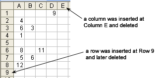
‘ The sample below demonstrates the problems and solution with the last cell, column and row.
’ To begin with, key in the values; insert a row at row 9 and delete it; insert a column at E and also delete it
ActiveSheet.Cells.SpecialCells(xlLastCell).Row     ' returns 9
ActiveSheet.Cells.SpecialCells(xlLastCell).Column  ' returns 5
ActiveSheet.UsedRange.Rows.Count                   ' returns 8
ActiveSheet.Cells.SpecialCells(xlLastCell).Row     ' returns 8, after correction from Rows.Count
Application.CountA (Range("A:B"))                  ' returns 8
ActiveSheet.Cells(Rows.Count, 1).End(xlUp).Offset(1, 0).Row  ' returns 9
ActiveSheet.UsedRange.Address      ‘ returns string $A$2:$D$8 and corrects the last cell location

Return To Top

' Find number of rows in the UsedRange in another worksheet
Dim mySheet As Worksheet
Set mySheet = Sheets("Sheet2")
MsgBox "number of used rows are " & mySheet.UsedRange.Rows.Count

' Displays row of first and last cell in a selection, then input sum formula of selected range in a column to E1.
It uses the public UDF to find the Column letter. The example works only with selection in one column.
Sub RowOfFirstAndLastCell()
  FirstRow = Selection(1).Row
  LastRow = Selection(Selection.Count).Row
  MsgBox "you select from row " & FirstRow & " to " & LastRow

  cL = ColumnLetter(ActiveCell.Column)
  Range("E1").Formula = "=sum(" & cL & FirstRow & ":" & cL & LastRow & ")"
End Sub

Public Function ColumnLetter(ColumnNumber As Long) As String
    Const OffsetLng_c As Long = 64
    ColumnLetter = VBA.Chr$(ColumnNumber + OffsetLng_c)
End Function

' To select all the cells that are filled with formula
Cells.SpecialCells(xlCellTypeFormulas, xlCellTypeLastCell).Activate

Return To Top

' Place the cursor on the last cell in Column A

Cells(Cells.Rows.Count,"A").End(xlUp).Select

' Place the cursor 2 cells below the last entry in column A

Cells(rows.count,1).End(xlup)(3).Select

' Can use as Private Sub in your sheet module.
' Define the named range "MyRange" to all data in Column A (includes blanks) each time the worksheet recalculates
Range("A1", Range("A65536").End(xlUp)).Name = "MyRange"



’ This defines a dynamic range in Column A, but  it does not include blanks
Range("A1", Range("A1").End(xlDown)).Name = "MyRange"

' This defines the named range "MyRange" to all your data range each time the particular worksheet recalculates

Range(Range("IV1").End(xlToLeft), Range("A65536").End(xlUp)).Name = "MyRange"

' This selects the bottom last cell in a named range
Dim myRng As Range

Set myRng = Sheets("Sheet1").Range("MyRange")

With myRng

   .Parent.Select

   .Cells(.Cells.Count).Select

End With

' This UDF finds the letter of the Column where your cursor is pointing at.
' Further below are other ways of finding the column's letter

Public Sub Test()

   VBA.MsgBox ColumnLetter(ActiveCell.Column)

End Sub

Public Function ColumnLetter(ColumnNumber As Long) As String

   Const OffsetLng_c As Long = 64

   ColumnLetter = VBA.Chr$(ColumnNumber + OffsetLng_c)

End Function

' Find the column's letter thru an input box
Dim myCell As Range, iC As String
Set myCell = Application.InputBox(prompt:="Click on a cell: ", Type:=8)
iC = myCell.EntireColumn.Address(False, False)
iC = Left(iC, InStr(1, iC, ":") - 1)
MsgBox ("Column's letter is: " & iC)


' Get the active cell's column name
Dim Name$
Name = ActiveCell.Address
MsgBox "you selected the column " & Left(Right(Name, Len(Name) - 1), _
InStr(Right(Name, Len(Name) - 1), "$") - 1)


' Get the active cell's column name
Dim mCol As String
mCol = Split(ActiveCell(1).Address(1, 0), "$")(0)
MsgBox mCol


' UDF to convert a column's number to a letter
Function ConvertColNumToLetter(iCol As Integer) As String
Dim iAlpha As Integer, iRemainder As Integer
iAlpha = Int(iCol / 27)
iRemainder = iCol - (iAlpha * 26)
  If iAlpha > 0 Then
     ConvertColNumToLetter = Chr(iAlpha + 64)
  End If

  If iRemainder > 0 Then
     ConvertColNumToLetter = ConvertColNumToLetter & Chr(iRemainder + 64)
  End If
End Function


' UDF to convert a column's number to a letter
Function ColumnLetter(Col As Long)
Dim sColumn As String

On Error Resume Next
sColumn = Split(Columns(Col).Address(, False), ":")(1)
On Error GoTo 0
ColumnLetter = sColumn
End Function


' This UDF finds the value or text of the last used cell in any single column
Public Function LastInColumn(rng As Range) As Variant

   LastInColumn = Cells(Rows.Count, rng(1).Column).End(xlUp).Value

End Function

=LastInColumn(A:A)    ‘ enter it in a cell

Return To Top

' Select an entire range of contiguous cells in a Column

Range("A1", ActiveSheet.Range("A1").End(xlDown)).Select

' Another way to select an entire range of contiguous cells in a Column
Range("A1:" & ActiveSheet.Range("A1").End(xlDown).Address).Select

' Either way will select an entire range of non-contiguous cells in a Column

Range("A1", ActiveSheet.Range("A65536").End(xlUp)).Select

Range("A1:" & ActiveSheet.Range("A65536").End(xlUp).Address).Select

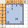
' CurrentRegion method selects a rectangular range of cells around a cell. The range selected by the CurrentRegion

  is an area bounded by any combination of blank rows and blank columns
ActiveSheet.Range("A1").CurrentRegion.Select

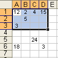
' CurrentRegion method will not work on pictorial example below because of the blank line on Row 4, these lines will.

lastcol = ActiveSheet.Range("A1").End(xlToRight).Column

lastrow = ActiveSheet.Cells(65536, lastcol).End(xlUp).Row

ActiveSheet.Range("A1", ActiveSheet.Cells(lastrow, lastcol)).Select

' Either of the methods below will select a range of contiguous data from A1 down (to the last cell with value),

then continues to select a range of contiguous data to its right.

ActiveSheet.Range("A1", ActiveSheet.Range("A1") _

  .End(xlDown).End(xlToRight)).Select             

ActiveSheet.Range("A1:" & ActiveSheet.Range("A1"). End(xlDown). _
  End(xlToRight).Address).Select

' Select the entire row of the last used cell in column A

Cells(Cells.Rows.Count, "A").End(xlUp).EntireRow.Select

' Select the entire row of the last used cell in any column
Cells.SpecialCells(xlLastCell).EntireRow.Select


' Select from activecell down to the last used row in the column
Dim rng As Range
  With ThisWorkbook.ActiveSheet
     Set rng = .Range(ActiveCell, LastCellInColumn(ActiveCell))
     rng.Select
  End With
Set rng = Nothing


Function LastCellInColumn(rngInput As Range) As Range
Dim lngCount As Long, rngWorkRange As Range, rngCell As Range
Set rngWorkRange = rngInput.Columns(1).EntireColumn
  With rngWorkRange
     lngCount = .Rows.Count
     Set rngCell = .Cells(lngCount, 1)
  End With

  If IsEmpty(rngCell) Then
     Set LastCellInColumn = rngCell.End(xlUp)
  Else
     Set LastCellInColumn = rngCell
  End If
End Function

Return To Top

Some Excel functions for last cell in a column:

‘ These three examples find the last used row number in column A. SUMPRODUCT is an array formula

=SUMPRODUCT(MAX((ROW(A1:A65535))*(A1:A65535<>"")))

‘ These two examples find only the numerical value of the last used cell in column A
=LOOKUP(9.99999999999999E+307,A:A)
=INDEX(A:A,MATCH(9.99999999999999E+307,A:A))

‘ This finds only  the text string of the last used cell in column A
=INDEX(A:A,MATCH(REPT("z",255),A:A,1),1)

’ Enter as an array formula, which finds only  the text string of the last used cell in column A
= INDEX($A$1:$A$65535,MAX(IF(ISTEXT($A$1:$A$65535),ROW($A$1:$A$65535))),1)

‘ Find row number of the last used cell (that contain only numerical value) in column A
=MATCH(9.99999999999999E+307,A:A)

‘ Find row number of the last used cell (that contain only text string) in column A
=MATCH(REPT("z",255),A:A)

‘ Fhese functions can find either text or numerical value of the last used cell in column A
=INDIRECT("A"&SUMPRODUCT(MAX((ROW(A1:A65535))*(A1:A65535<>""))))

’ Enter as an array formula, which finds either text or value of the last used cell in column A
=INDIRECT("A"&MAX(IF(NOT(ISBLANK(A1:A65535)),ROW(1:65535))))

Return To Top

Deleting, Adding and Hiding Rows, Columns and Sheets

’  This deletes all the rows after the active row until row 65536
Range(ActiveCell.Row + ActiveCell.Rows.Count & ":" & Cells.Rows.Count).Delete

’  This is same as choosing Range(Cells(1,i+1), "IV65536").Delete
Range(Cells(1, ActiveCell.Column + ActiveCell.Columns.Count), _
   Cells(Cells.Rows.Count, Cells.Columns.Count)).Delete

’  Delete rows after last cell used in column A
Range(Cells(Rows.Count, 1).End(xlUp).Offset(1), Cells(Rows.Count, 1)).EntireRow.Delete

‘ Delete all the blank rows in the active sheet
Dim LastRow As Long, i As Long
LastRow = Cells(ActiveSheet.UsedRange.Rows.Count, ActiveCell.Column).Row

Application.ScreenUpdating = False
  For i = LastRow To 1 Step -1
    If Application.CountA(Rows(i)) = 0 Then Rows(i).Delete
  Next i

‘ Delete all the hidden rows in the active sheet, using For next loop
Dim i As Long, LastRow As Long
LastRow = Cells(ActiveSheet.UsedRange.Rows.Count, ActiveCell.Column).row

  For i = LastRow To 1 Step -1

    If Rows(i).Hidden Then

      Rows(i).Hidden = False

      Rows(i).Activate

      Selection.EntireRow.Delete

    End If

  Next i

Return To Top

’ Delete all the hidden rows in the active sheet without using For next loop
Dim r As Range, k As Range

With ActiveSheet

  Set r = .Range("A1:A" & .Cells.SpecialCells(xlCellTypeLastCell).row)

  Set k = r.SpecialCells(xlCellTypeVisible)

  r.EntireRow.Hidden = False

  k.EntireRow.Hidden = True

  r.SpecialCells(xlCellTypeVisible).EntireRow.Delete

  r.EntireRow.Hidden = False

  Set r = Nothing
  Set k = Nothing

End With

' Delete rows where the entry in column A matches the row above it

Dim r As Long, lastrow As Long

lastrow = Cells(Rows.Count, 1).End(xlUp).Row

  For r = lastrow To 2 Step -1

    If Cells(r, 1) = Cells(r - 1, 1) Then Rows(r).EntireRow.Delete

  Next r

' Delete rows with duplicate data in the active column

Dim ActCol As Integer, Val As Variant, Rng As Range, i As Long

ActCol = ActiveCell.Column

Set Rng = ActiveSheet.UsedRange.Rows

i = 0

For i = Rng.Rows.Count To 1 Step -1

Application.ScreenUpdating = False

  Val = Rng.Cells(i, ActCol).Value

  If Application.WorksheetFunction.CountIf(Rng.Columns(ActCol), Val) > 1 Then

     Rng.Rows(i).EntireRow.Delete

     i = i + 1

  End If

Next i

Application.ScreenUpdating = True

Return To Top

’ Delete filtered rows with string “#N/A” found in column C
’ This example uses Offset to move the UsedRange range down one row to avoid including the headers, and resize
' the range to number of rows – 1)
ActiveSheet.Cells(1, 1).AutoFilter Field:=3, Criteria1:="#N/A"

Application.DisplayAlerts = False

On Error Resume Next

ActiveSheet.UsedRange.Offset(1, 0).Resize(ActiveSheet.UsedRange.Rows.Count - 1).Rows.Delete
Application.DisplayAlerts = True

Selection.AutoFilter Field:=3

' Delete rows that contain string name  “william”  in column B
Dim rng As Long

For rng = 1 To 100

  If Cells(rng, 2).Value = "william" Then
     Cells(rng, 2).EntireRow.Delete

     rng = rng + 1

  End If

Next rng

‘ Another method of deleting rows that contain string “william”  in column B
Dim rng As Range

Set rng = Range("B2:B" & Cells(65536, "B").End(xlUp).Row)

If ActiveSheet.AutoFilterMode Then Cells.AutoFilter

   Columns("B").AutoFilter Field:=1, Criteria1:="= william"

   On Error Resume Next

   r.SpecialCells(xlCellTypeVisible).EntireRow.Delete

   On Error GoTo 0
End If

Return To Top

’ Delete all rows that have a negative number in column B
Dim Rng As Range

Dim rowsCnt As Long, n As Long

With ActiveSheet

    rowsCnt = .UsedRange.Rows.Count

    Set Rng = .Range(.Cells(1, 2), .Cells(rowsCnt, 2))

End With

For n = rowsCnt To 1 Step -1

    If Rng.Cells(n, 1).Value < 0 Then

       Rng.Cells(n, 1).EntireRow.Delete

    End If

Next n

‘ Delete rows when date data dd/mm/yyyy in column 2 does not contain “2008”, four places from the Right
Dim i As Long, lastrow As Long
lastrow = Cells(65536, 2).End(xlUp).Row
For i = lastrow To 1 Step -1
  If Right(CStr(Cells(i, 2).Value), 4) <> "2008" Then
    Rows(i).Delete
  End If
Next

' Delete rows based on a specified criteria.
Dim tableSEL As Range, colSEL As Long, criteriaSEL
On Error Resume Next
  With Selection
    If .Cells.Count > 1 Then   ' number of cells count
        Set tableSEL = Selection
    Else
        Set tableSEL = .CurrentRegion  ' determine the table range
        On Error GoTo 0
    End If
  End With

    If tableSEL Is Nothing Or tableSEL.Cells.Count = 1 Or _
        WorksheetFunction.CountA(tableSEL) < 2 Then   ' determine if table range is valid
        MsgBox "could not find your table range.", vbCritical, ""
        Exit Sub
    End If

    ' get the criteria in the form of text or number
    criteriaSEL = Application.InputBox(Prompt:="Type in the criteria that you " _
      & "want the macthing rows to be deleted. If the criteria is in a cell, " _
      & "point your mouse pointer to that cell", _
      Title:="delete rows based on criteria, text or number", Type:=1 + 2)
    If criteriaSEL = "False" Then Exit Sub   ‘ exit sub if you select Cancel
    colSEL = Application.InputBox(Prompt:="Type in the column number where criteria ” _
      & “can be found", Title:="delete rows based on criteria, text or number", Type:=1)
    If colSEL = 0 Then Exit Sub  ' cancelled
   
    ActiveSheet.AutoFilterMode = False   ' remove any existing AutoFilters
    tableSEL.AutoFilter Field:=ColSEL, Criteria1:=criteriaSEL ' filter table based on criteriaSEL using the relative column position stored in lCol
    tableSEL.Offset(1, 0).SpecialCells(xlCellTypeVisible).EntireRow.Delete  ' delete all rows that are NOT hidden by AutoFilter
On Error GoTo 0

Return To Top

’  Hide row 2 to 4, 6 to 8, 10 to 12 and so forth, stepping through every 4 rows
Dim i As Long, n As Long
n = Cells(65536, 1).End(xlUp).Row
For i = 1 To n Step 4
    Range(Cells(i + 1, 1), Cells(i + 3, 1)).EntireRow.Hidden = True
Next i

‘ Using command button to toggle hide/unhide specified columns (6 columns to the Right from column 7)
If CommandButton1.TopLeftCell.Offset(0, 5).Resize(, 6).EntireColumn.Hidden = False Then
   CommandButton1.TopLeftCell.Offset(0, 5).Resize(, 6).EntireColumn.Hidden = True
Else: CommandButton1.TopLeftCell.Offset(0, 5).Resize(, 6).EntireColumn.Hidden = False
End If

' Delete all worksheets except the sheet named “MySheet”
Dim Sht As Object
Application.DisplayAlerts = False
 For Each Sht In Sheets
    If Not Sht.Name = "MySheet" Then
      On Error Resume Next
      Sht.Delete
    End If
 Next Sht

Return To Top

’ Delete all worksheets except the first sheet “Sheet1” and second sheet “Sheet2”
Dim I As Integer
Application.ScreenUpdating = False
Application.DisplayAlerts = False
 For I = ActiveWorkbook.Worksheets.Count To 1 Step -1
   If Worksheets(I).Name <> "Sheet1" And Worksheets(I).Name <> "Sheet2" Then
   Worksheets(I).Delete
 Next I
Application.ScreenUpdating = True

‘ Delete all empty sheets
Dim sh As Worksheet
For Each sh In ThisWorkbook.Worksheets
    If Application.WorksheetFunction.CountA(sh.Cells) = 0 Then
       Application.DisplayAlerts = False
       sh.Delete
    Else
       If Worksheets.Count = 1 Then
         Exit For
         Application.DisplayAlerts = True
       End If
    End If
Next

' Add one row after every alternating row, fill them with color and formula (eg, A2=B1, A4=B2, and if B2 is blank, leave
A4 as blank, and so on), then convert formula to values.
Dim i As Long, LastRow As Long, cel As Range
LastRow = Cells(ActiveSheet.UsedRange.Rows.Count, ActiveCell.Column).Row
For i = LastRow To 2 Step -1
   Rows(i).Insert Shift:=xlDown
Next i

ActiveSheet.UsedRange.SpecialCells(xlCellTypeBlanks).Select
Selection.Interior.ColorIndex = 5
Selection.FormulaR1C1 = "=IF(R[-1]C[1]="""","""",R[-1]C[1])"

For Each cel In Selection
  cel = cel.Value
Next cel

Return To Top

Working around Cells in the Worksheet

‘ Either of these select the same cell on the active Worksheet
ActiveSheet.Cells(3, 2).Select
ActiveSheet.Range("B3").Select


' Select Cell B3 in Sheet2 in the same Workbook
Application.Goto ActiveWorkbook.Sheets("Sheet2").Cells(3, 2)


‘ Select Cell B3 in Sheet2 in the another workbook “BOOK2.XLS”
Application.Goto Workbooks("BOOK2.XLS").Sheets("Sheet2").Cells(3, 2)


‘ Select a Range of cells (B3:C10) on the Active Worksheet
ActiveSheet.Range(Cells(3, 2), Cells(10, 3)).Select


‘ Select a Range of Cells on another worksheet in the same Workbook
Application.Goto ActiveWorkbook.Sheets("Sheet2").Range("B3:C10")


‘ Either line of code will select a Range of cells on a Worksheet in a different Workbook “BOOK2.XLS”
Application.Goto Workbooks("BOOK2.XLS").Sheets("Sheet1").Range("B3:C10")
Workbooks("Book2.xls").Worksheets("Sheet1").Range(Cells(3, 2), Cells(10, 3)).Select


‘ Select a named Range of cells “myRange” on a Sheet 1in a different Workbook “BOOK2.XLS”
Workbooks("Book2.xls").Worksheets("Sheet1").Range("myRange").Select


‘ Select a cell relative to another cell (here is selecting C5 relative to A2)
ActiveSheet.Cells(2, 1).Offset(5, 3).Select


‘ Select a named Range of cells “myRange” and Resize the Selection
ActiveSheet.Range("myRange").Select
Selection.Resize(Selection.Rows.Count + 5, Selection.Columns.Count).Select


‘ Select a named Range of cells “myRange”, Offset it (3 cells down and 2 cells to the Right), and then Resize it (extend
the selection by 4 rows down and 5 columns to the Right
ActiveSheet.Range("myRange").Select
Selection.Offset(3, 2).Resize(Selection.Rows.Count + 4,Selection.Columns.Count + 5).Select


' Select the Union of  two or more Named Ranges (note both ranges must be on the same worksheet)
Application.Union(Range("myRange"), Range("testRange")).Select

Return To Top

‘ Select the blank Cell at bottom of  Column A of contiguous data
ActiveSheet.Range("A1").End(xlDown).Offset(1,0).Select


‘ Select an entire Range of contiguous Cells in Row 1
ActiveSheet.Range("A1", ActiveSheet.Range("A1").End(xlToRight)).Select


‘ Select an entire Range of non-contiguous Cells in Row 1
ActiveSheet.Range("A1", ActiveSheet.Range("IV1").End(xlToLeft)).Select


' Select a rectangular Range of contiguous Cells
ActiveSheet.Range("A1", ActiveSheet.Range("A1").End(xlDown).End(xlToRight)).Select


' Select a rectangular Range of non-contiguous Cells which CurrentRegion method will not work
Dim lastRow As Long, lastCol As Long
lastCol = ActiveSheet.Range("IV1").End(xlToLeft).Column
lastRow = Cells(ActiveSheet.UsedRange.Rows.Count, ActiveCell.Column).Row
ActiveSheet.Range("A1", ActiveSheet.Cells(lastRow, lastCol)).Select

     ' or using this:
ActiveSheet.Range("A1:" & ActiveSheet.Cells(lastRow, lastCol).Address).Select


' Select multiple non-contiguous Columns of varying length using Union method (here is Column A & C)
Dim a As Range, c As Range
Set a = ActiveSheet.Range("A1", ActiveSheet.Range("A65536").End(xlUp))
Set c = ActiveSheet.Range("C1", ActiveSheet.Range("C65536").End(xlUp))
Union(a, c).Select


' Sets the value of the merged range at Cells(2,3) from A2
Set ma = Range("A2").MergeArea
    ma.Value = "888"
    ma.Cells(2, 3).Value = "889"


‘  Delete all duplicate data in column A
Dim cell As Range, Last As Double, nonDupl As New Collection
On Error GoTo ErrHandler
Last = Range("A65536").End(xlUp).Row
  For Each cell In Range("A1:A" & Last)
    If Not IsEmpty(cell) Then
       nonDupl.Add cell.Value, CStr(cell.Value)
    End If
  Next cell
  Exit Sub
ErrHandler:
  cell.Clear
  Resume Next

Return To Top

A note on COPY, CUT, PASTE in VBA

Below are the commonly used Excel functions (Copy, Cut, Paste Special methods), now you see it in VBA.

Copy method
Sheet1.Range("A1").Copy Destination:=Sheet2.Range("A2")

Advance Copy Example
' this will copy all your values in your active column in Sheet2 to the column from row 2 all the way down in Sheet1 (when one cell above it is the last empty cell leftward from cell IV1).   
Sheets(2).Range(ActiveCell.Address, _ Cells(Rows.Count, ActiveCell.Column).End(xlUp).Address).Copy _ Sheets(1).Range("IV1").End(xlToLeft).Offset(1, 1) 

Sheet1

Sheet2

Cut method
Sheet1.Range("A1").Cut Destination:=Sheet2.Range("A2")

Copy and PasteSpecial method
expression.PasteSpecial(Paste, Operation (optional), SkipBlanks (optional TRUE/FALSE), Transpose (optional TRUE/FALSE)

Example:
Sheet1.Range("A1").Copy
Sheet2.Range("A1").PasteSpecial Paste:= xlPasteValues, Operation:=xlNone, SkipBlanks:=False, TRANSPOSE:=False
Application.CutCopyMode=False      ' clears clipboard

    Paste option can be one of these :
xlPasteAll (default), xlPasteAllExceptBorders, xlPasteColumnWidths, xlPasteComments, xlPasteFormats, xlPasteFormulas, xlPasteFormulasAndNumberFormats, xlPasteValidation,  xlPasteValues, xlPasteValuesAndNumberFormats

    Operation (optional) can be :
xlNone (default), xlPasteSpecialOperationAdd, xlPasteSpecialOperationDivide, xlPasteSpecialOperationMultiply, xlPasteSpecialOperationSubtract

    SkipBlanks  is Optional. The default value is False.

    Transpose  is Optional. The default value is False.


Copy Formula method
Sheet1.Range("A1").Formula= Sheet2.Range("A2").Formula